McGraw.Hill PIC Robotics A Beginners Guide to Robotics Projects Using the PIC Micro eBook-LiB Part 8 ppt
Bạn đang xem bản rút gọn của tài liệu. Xem và tải ngay bản đầy đủ của tài liệu tại đây (2.62 MB, 20 trang )
Vehicle A, if both sensors are evenly illuminated by a light source, will speed
up and, if possible
,
run into the light source. However, if the light source is off
to one side, the sensor on the side of the light source will speed a little faster
than the sensor/motor on other side. This will cause the vehicle to veer away
from the light source (see F
ig
.
9.7).
Vehicle B, if both sensors are evenly illuminated by a light source, will speed
up and, if possible, run into the light source (same as vehicle A). If the light
source is off to one side
,
vehicle B will turn toward the light source (see Fig. 9.7).
Braitenberg Vehicles 127
Figure 9.2 Graph of positive pro-
portional transfer function. As
sensor output increases, motor
output increases.
Figure 9.3 Graph of negative
proportional transfer function.
As sensor output increases,
motor output decreases.
Figure 9.4 Graph of digital transfer function. As sensor output increases, output
remains unchanged until threshold is reached, then output switches full on.
128 Chapter Nine
Figure 9.5 Graph of gaussian function. As sensor output increases, output
follows a gaussian curve.
Figure 9.6 Wiring of two Braitenberg vehicles labeled A and B.
Negative proportional neural setups would show the opposite behavior.
Building Vehicles
It’s time to put the theory to the test and see if it works. Let’s assemble the
materials needed to build a vehicle. The photovore’s basic operating procedure
is like Walter’s robot. It tracks and follows a light source.
The base of the vehicle is a sheet of aluminum 8 in long by 4 in wide by
1
�
8
in thick. We will use two gearbox motors for propulsion and steering and one
multidirectional front wheel.
We will try a new construction method with this robot. Instead of securing the
gearbox motors with machine screws and nuts, we will use 3M’s industrial
brand double-sided tape
.
This double-sided tape, once cured, is as strong as pop
rivets. I tried to separate a sample provided by 3M. It consisted of two flat pieces
of metal secured with the tape. Even when I used pliers, it was impossible. 3M
states that the tape requires 24 h to reach full strength.
You may not achieve the
full-strength capability of the tape unless you follow the 3M procedure.
Braitenberg Vehicles 129
Figure 9.7 Function of A and B Braitenberg vehicles.
The gearbox motor is a 918D type (see Fig. 9.8). The gearbox motor at the
top of the picture has an orange cowl that is covering the gears. Notice the flat
mounting bracket that is perfect for securing to the vehicle base. The double-
sided tape is cut lengthwise to fit the base of bracket to the gearbox motor. The
exposed side of the tape is immediately secured to the gearbox motor bracket.
Then the motor is positioned on the bottom of the vehicle base, the protective
covering of the tape is removed, and the gearbox motor is firmly placed onto
the bottom of the vehicle base (see Fig. 9.9).
The second gearbox motor is secured to the other side in a similar manner.
Back wheels
The shaft diameter of the gearbox motor is a little too small to make a good
friction fit to the rubber wheel. To beef up the diameter, cut a small 1- to 1.5-
in length of the 3-mm tubing; see Parts List. Place the tubing over the gearbox
motor shaft, and collapse the tubing onto the shaft, using pliers. There is a
small cutaway on the gearbox motor shaft (see Fig. 9.10). If you can collapse
the tubing into this cutaway, you will create a strong fit between the shaft and
the tubing that will not pull off easily (see Fig. 9.11).
The tubing adds to the diameter of the shaft and will make a good friction
fit with the rubber wheels (see Fig. 9.12). Simply push the center holes of the
wheels onto the tubing/shaft, and you are finished.
130 Chapter Nine
Figure 9.8 A 918D 100:1 Gearbox motor.
Figure 9.9 3M double-sided tape is used to secure gearbox motor to base
of vehicle
.
Braitenberg Vehicles 131
Figure 9.10 Gearbox motor showing cutaway on output shaft.
Figure 9.11 A 1
1
�
2
-in length of 3-mm-diameter tubing attached to gearbox
motor shaft.
Front wheels
Steering is accomplished by turning on or off the gearbox motors. For instance,
turning on the right while the left gearbox motor is off will turn the vehicle to the
left,
and vice versa.
In similar vehicles many times the robotists will forgo front
wheels entirely and use a skid instead.
This allows the vehicle to turn without
concern about the front wheels pivoting and turning in the proper direction
The multidirectional wheel accomplishes much the same thing as a skid,
but
does so with less resistance
.
F
igure 9.13 shows the multidirectional wheel.
It
is constructed using rollers around its circumference that allow the wheel to
rotate forward and move sidew
a
ys without turning
.
132 Chapter Nine
Figure 9.12 Rubber wheel used to friction fit onto gearbox motor shaft.
The multidirectional wheel is attached using a basic U-shaped bracket (see
Fig. 9.14). The bracket is secured to the front of the vehicle base using the 3M
double-sided tape. The multidirectional wheel is secured inside the U bracket
using a small 2.25-in piece of
1
4
-20 threaded rod and two machine screw nuts
(see Fig. 9.15).
With the motors and the multidirectional wheel mounted, we are ready
for the electronics. Figure 9.16 shows the underside of the Braitenberg
vehicle at this point. I drilled a
1
4
-in hole in the aluminum plate to allows
wires from the gearbox motors underneath the robot to be brought top-
side.
The schematic for the electronic circuit is shown in Fig. 9.17. I built the cir-
cuit on two small solderless breadboards. You can do the same or hardwire the
components to a PC board. The circuit is pretty straightforward. The gearbox
motors require a power supply of 1.5 to 3.0 V. Rather than place another volt-
age regulator into the circuit, I wired three silicon diodes in series off the 5-V
dc power. The voltage drop across each diode is approximately 0.7 V. Across the
three series diodes (0.7
3 2.1
V) equals approximately 2.1
V
. If we subtract
this voltage drop from our regulated 5-V dc power supply, we can supply
approximately 3 V dc to the gearbox motors.
Braitenberg Vehicles 133
Figure 9.13 Multidirectional wheel.
Figure 9.14 Drawing of U bracket
for multidirectional wheel.
CdS photoresistor cells
As with Walter’s turtle-type robot, we use two CdS photoresistor cells. The CdS
photoresistors (see F
ig
.
9.18) used in this robot have a dark resistance of about
100 k�
and a light resistance of 10 k�. The CdS photoresistors typically have
large variances in resistance between cells
. It is useful to use a pair of CdS cells
for this robot that matches
,
as best as one can match them,
in resistance.
Since the resistance values of the CdS cells can vary so greatly, it’s a good
idea to buy a few more than you need and measure the resistances to find a
pair whose resistances are close
.
There are a few w
ays you can measure the
resistance. The simplest method to use a volt-ohmmeter, set to ohms. Keep the
light intensity the same as you measure the resistance. Choose two CdS cells
that are closely matched within the group of CdS cells you have
.
Figure 9.15 Multidirectional wheel and U bracket attached to vehicle
base.
Figure 9.16 Underside of Braitenberg vehicle showing wheels and gearbox
motor drive.
134
RB7
RB6
RB5
RB4
RB3
RB2
RB1
RB0/INT
RA4/TOCKI
RA3
RA2
RA1
RA0
13
12
11
10
9
8
7
6
3
2
1
18
17
CdS
Photocell
CdS
Photocell
Sensor 1Sensor 2
V1
50 kΩ
V1
50 kΩ
D1
1N4002
R2
330 Ω
Q1
2N3904
DC
Motor
D2
1N4002
R3
330 Ω
Q1
2N3904
DC
Motor
MCLR'
OSC 1
OSC 2
+3 V Vcc+3 V Vcc
VDD
VSS
5
4
16
15
U1
14
R1
4.7 k Ω
C1
.1 µF
X1
4 MHz
+5 V Vcc
PIC 16F84
C4
10 µF
20 V
C5
100 µF
20 V
U2
LM2940
D3
1N4002
D4
1N4002
D5
1N4002
+3 V
+5 V
6 V
+
I
1
2
3
O
R
C2
.1 µF
C3
.1 µF
++
Figure 9.17 Schematic of Braitenberg vehicle.
135
136 Chapter Nine
Figure 9.18 CdS photoresistor
cell.
The second method involves building a simple PIC 16F84 circuit connected
to an LCD display. The advantage of this circuit is that you can see the
response of the CdS cells under varying light conditions. In addition, you can
see the difference in resistance between the CdS cells when they are held
under the same illumination. This numeric difference of the CdS cells under
exact lighting is used as a fudge factor in the final turtle program. If you just
test the CdS cells with just an ohmmeter, you will end up using a larger fudge
factor for the robot to operate properly.
The schematic for testing the CdS cells is shown in Fig. 9.19. The circuit,
built on a PIC Experimenter’s Board, is shown in Fig. 9.20. The PicBasic Pro
testing program follows:
‘CdS cell test
‘PicBasic Pro program
‘Serial communication 1200 baud true
‘Serial information sent out on port b line 0
‘Read CdS cell #1 on port b line 1
‘Read CdS cell #2 on port b line 7
v1 var byte ‘Variable v1 holds CdS #1 information
v2 var byte ‘Variable v2 holds CdS #2 information
Pause 1000 ‘Allow time for LCD display
main:
pot portb.1,255,v1 ‘Read resistance of CdS #1 photocell
pot portb.7,255,v2 ‘Read resistance of CdS #2 photocell
‘Display information
serout portb.0,1,[$fe,$01] ‘Clear the screen
Braitenberg Vehicles 137
LCD Display
V1
100KΩ
V2
100KΩ
CdS
Cell
CdS
Cell
C2
.1µF
50V
C3
.1µF
50V
SW4
C1
.1µF
R1
4.7KΩ
U1
+5V
X1
4MHz
4
16
15
PIC 16F84
5
VSS
VDD
17
18
1
2
3
6
7
8
9
10
11
12
13
RB7
RB6
RB5
RB4
RB3
RB2
RB1
RB0/INT
RA4/TOCKI
RA3
RA2
RA1
RA0
14
MCLR'
OSC1
OSC2
Serial Line
+5V
Gnd
Figure 9.19 Schematic of test circuit to match CdS cells for use in Braitenberg vehicle.
pause 25
serout portb.0,1,[”CdS 1 = ”]
serout portb.0,1,[#v1]
serout portb.0,1,[$fe,$c0] ‘Move to line 2
pause 5
serout portb.0,1,[”CdS 2 = ”]
serout portb.0,1,[#v2]
pause 100
goto main
Notice in Fig. 9.20 that CdS cell 1 is reading 37 and CdS cell 2 is reading 46
under identical lighting. Keep in mind, this is a closely matched pair of CdS
cells. We can use a fudge factor of ±15 points, meaning that as long as the read-
ings between cells vary from each other by ω15 points
, the microcontroller will
consider them numerically equal.
Trimming the sensor array
If you are using the Experimenter’s Board, you can trim and match the CdS
cells to one another. Doing so allows you to reduce the fudge factor and pro-
duces a crisper response from the robot.
Typically one CdS cell resistance will be lower than that of the other CdS
cell. To the lower-resistance CdS cell add a 1-k
� (or 4.7-k�) trimmer poten-
tiometer in series (see Fig. 9.21). Adjust the potentiometer (trim) resistance
until the outputs shown on the LCD displa
y equal each other. Trim the CdS
cell under the same lighting conditions in which the robot will function. The
138 Chapter Nine
Figure 9.20 Test circuit built on PIC Experimenter’s Board.
LCD Display
V1
100KΩ
V2
100KΩ
CdS
Cell
CdS
Cell
C2
.1µF
50V
C3
.1µF
50V
SW4
C1
.1µF
R1
4.7KΩ
U1
+5V
X1
4MHz
4
16
15
PIC 16F84
5
VSS
VDD
17
18
1
2
3
6
7
8
9
10
11
12
13
RB7
RB6
RB5
RB4
RB3
RB2
RB1
RB0/INT
RA4/TOCKI
RA3
RA2
RA1
RA0
14
MCLR'
OSC1
OSC2
Serial Line
+5V
Gnd
1KΩ
V3
Figure 9.21 Schematic of test circuit with trimmer potentiometer
.
Braitenberg Vehicles 139
reason for this is that when the light intensity varies from that nominal point
to which you’ve trimmed the CdS cell, the responses of the individual CdS cells
to changes in light intensity also vary from one another and then are not as
closely matched.
PIC 16F84 microcontroller
The 16F84 microcontroller used in this robot simulates two neurons. Each
neuron’s input is connected to a CdS cell. The output of each neuron activates
one gearbox motor.
In the program I put in a fudge factor, or range, over which the two CdS cells
can deviate from one another in resistance readings and still be considered
equal. If the robot doesn’t travel straight ahead when the two CdS cells are
equally illuminated, you can increase the range until it does.
PicBasic Compiler program
‘Braitenberg vehicle 1
start:
pot 1, 255,b0
pot 2, 255,b1
If b0 = b1 then straight
if b0 > b1 then left
if b1 > b0 then right
straight:
high 3: high 4
goto start
left:
b2 = b0 - b1
if b2 > 15 then left1
goto straight
left1:
high 3: low 4
goto start
right:
b2 = b1 - b0
if b2 > 15 then right1
goto straight
right1:
high 4: lo3
goto start
Testing
‘Read CdS cell # 1
‘Read CdS cell # 2
‘Compare numerical values +/- 15
‘If greater than 15 turn left
‘If not go to straight subroutine
‘Turn left
‘Motor control
‘Compare numerical values +/- 15
‘If greater then 15 points
‘Turn toward the right
‘If not go straight
‘Turn right
‘Motor control
‘Do again
The finished robot is shown in F
ig
.
9.22.
F
or power I used 4 AA cell batteries.
I pointed one CdS cell to the left and the other to the right (see Fig. 9.23). To
140 Chapter Nine
Figure 9.22 Finished Braitenberg vehicle.
Figure 9.23 Close-up of CdS cells mounted in solderless breadboard.
Braitenberg Vehicles 141
test the robot’s function, I used a flashlight. Using the flashlight, I was able to
steer the mobile platform around by shining the flashlight on the CdS cells.
Second Braitenberg Vehicle (Avoidance Behavior)
Given the way the robot is currently wired, it is attracted to and steers toward
a bright light source. By reversing the wiring going to the gearboxes you can
create the opposite behavior.
Parts List
(1) Microcontroller (16F84)
(1) 4.0-MHz crystal
(2) 22-pF caps
(1) 0.1-F cap
(1) 100-F cap
(1) 10-F cap
(2) 0.1-F caps
(2) 330-,
1
4
-W resistors
(1) 4.7-k,
1
4
-W resistor
(2) CdS photoresistor cells (see text)
(2) 100:1 gearbox motors (918D)
(2) NPN transistors (2N3904)
(5) Diodes (1N4002)
(2) 2.25-in-diameter wheels
(1) Multidirectional wheel
(1) Voltage regulator (low drop-down voltage
5 V) (LM2940)
Miscellaneous items needed include 6-in length of 3-mm hollow tubing, alu-
minum 8 in 4 in
1
8
in thick,
2 solderless breadboards, 3M double-sided
tape, battery holder for 4 D batteries, 3-in
1
4
-20 threaded rod, and 2 machine
screw nuts.
This page intentionally left blank.
10
Chapter
Hexapod Walker
Legged walkers are a class of robots that imitate the locomotion of animals
and insects, using legs. Legged robots have the potential to transverse rough
terrains that are impassable by standard wheeled vehicles. It is with this in
mind that robotists are developing walker robots.
Imitation of Life
Legged walkers may imitate the locomotion style of insects, crabs, and some-
times humans. Biped walkers are still a little rare, requiring balance and a
good deal more engineering science than multilegged robots. A bipedal robot
walker is discussed in detail in Chap. 13. In this chapter we will build a six-
legged walker robot.
Six Legs—Tripod Gait
Using a six-legged model, we can demonstrate the famous tripod gait used by
the majority of legged creatures. In the following drawings a dark circle means
the foot is firmly planted on the ground and is supporting the weight of the
creature (or robot). A light circle means the foot is not supporting any weight
and is movable.
Figure 10.1A shows our walker at rest. All six feet are on the ground. From
the resting position our walker decides to move forward. To step forward, it
leaves lifts three of its legs (see Fig. 10.1B, white circles), leaving its entire
weight distributed on the remaining three legs (dark circles). Notice that the
feet supporting the weight (dark circles) are in the shape of a tripod. A tripod
is a very stable weight-supporting position.
Our w
alker is unlikely to fall over
.
The three feet that are not supporting any weight may be lifted (white circles)
and moved without disturbing the stability of the walker. These feet move for-
w
ard.
Copyright © 2004 The McGraw-Hill Companies. Click here for terms of use.
143
144 Chapter Ten
Figure 10.1 Sample biological tripod gait.
Figure 10.1C illustrates where the three lifted legs move. At this point,
the walker’s weight shifts from the stationary feet to the moved feet (see
Fig. 10.1D). Notice that the creature’s weight is still supported by a tripod
position of feet. Now the other set of legs moves forward and the cycle
repeats.
This is called a tripod gait,
because a tripod positioning of legs always sup-
ports the weight of the walker.
Three-Servomotor Walker Robot
The robot we will build is shown in Fig. 10.2. This walker robot is a compro-
mise in design, but allows us to build a six-legged walker using just three
servomotors. The three-servomotor hexapod walker demonstrates a true tri-
pod gait. It is not identical to the biological gait we just looked at, but close
enough.
This legged hexapod uses three inexpensive HS-322 (42-oz torque) servo-
motors for motion and one PIC 16F84 microcontroller for brains. The micro-
controller stores the program for walking, controls the three servomotors,
and reads the two sensor switches in front. The walking program contains
subroutines for walking forward and backward, turning right, and turning
left. The two switch sensors positioned in the front of the walker inform the
microcontroller of any obstacles in the walker’s path. Based on the feedback
from these switch sensors, the walker will turn or reverse to avoid obstacles
placed in its path.
Function
The tripod gait I programmed into this robot isn’t the only workable gait.
There are other perfectly usable gaits you can develop on your own. Consider
this walking program a working start point. To modify the program, it’s impor-
tant to understand both the program and robot leg functions. First let’s look at
the robot.
At the rear of the walker are two servomotors. One is identified as L for the
left side, the other as R for the right side. Each servomotor controls both the
front and back legs on its side. The back leg is attached directly to the horn of
the servomotor. It is capable of swinging the leg forward and backward. The
back leg connects to the front leg through a linkage. The linkage makes the
front leg follow the action of the back leg as it swings forward and back.
The third servomotor controls the two center legs of the walker. This servo-
motor rotates the center legs 20° to 30° clockwise (CW) or counterclockwise
(CCW), tilting the robot to one side or the other (left or right).
With this information we can examine how this legged robot will walk.
Moving Forward
W
e start in the rest position (see F
ig
.
10.3).
As before, each circle represents a
foot, and the dark circles show the weight-bearing feet. Notice in the rest posi-
tion, the center legs do not support any weight. These center legs are made to
be
1
/
8
in shorter than the front and back legs
.
In position A the center legs are rotated CW by about 25° from center posi-
tion. This causes the robot to tilt to the right. The weight distribution is now
on the front and back right legs and the center left leg
. This is the standard
tripod position as described earlier. Since there is no weight on the front and
back left legs, they are free to move forward as shown in the B position of
F
ig
. 10.3.
Hexapod Walker 145
Figure 10.2 Hexapod robot.
146 Chapter Ten
Figure 10.3 Forward gait for hexapod robot.
In the C position the center legs are rotated CCW by about 25° from center
position. This causes the robot to tilt to the left. The weight distribution is now
on the front and back left legs and the center right leg. Since there is no weight
on the front and back right legs, they are free to move forward, as shown in the
D position.
In position E the center legs are rotated back to their center position. The
robot is not in a tilted position so its weight is distributed on the front and
back legs. In the F position, the front and back legs are moved backward
simultaneously, causing the robot to move forward. The walking cycle can
then repeat.
Moving Backward
W
e start in the rest position (see F
ig. 10.4), as before. In position A the cen-
ter legs are rotated CW by about 25°
from center position.
The robot tilts
to the right. The weight distribution is now on the front and back right
legs and the center left leg
.
Since there is no weight on the front and back
left legs
,
they are free to move bac
kw
ard,
as shown in the B position of F
ig.
10.4.