Mechanics of Microelectromechanical Systems - N.Lobontiu and E.Garcia Part 1 docx
Bạn đang xem bản rút gọn của tài liệu. Xem và tải ngay bản đầy đủ của tài liệu tại đây (1.19 MB, 26 trang )
Mechanics of
Microelectro-
mechanical
Systems
This page intentionally left blank
Nicolae Lobontiu
Ephrahim Garcia
Mechanics of
Microelectromechanical
Systems
KLUWER ACADEMIC PUBLISHERS
NEW YORK, BOSTON, DORDRECHT, LONDON, MOSCOW
eBook ISBN: 0-387-23037-8
Print ISBN: 1-4020-8013-1
Print ©2005 Kluwer Academic Publishers
All rights reserved
No part of this eBook may be reproduced or transmitted in any form or by any means, electronic,
mechanical, recording, or otherwise, without written consent from the Publisher
Created in the United States of America
Boston
©2005 Springer Science + Business Media, Inc.
Visit Springer's eBookstore at:
and the Springer Global Website Online at:
To our families
This page intentionally left blank
TABLE OF CONTENTS
Preface
ix
STIFFNESS BASICS
1
1
1
6
14
21
43
58
60
INTRODUCTION
1
2
3
STIFFNESS DEFINITION
DEFORMATIONS, STRAINS AND STRESSES
4
5
6
7
MEMBERS, LOADS AND BOUNDARY CONDITIONS
LOAD-DISPLACEMENT CALCULATION METHODS:
CASTIGLIANO’S THEOREMS
COMPOSITE MEMBERS
PLATES AND SHELLS
Problems
MICROCANTILEVERS, MICROHINGES,
MICROBRIDGES
2
65
65
66
97
103
114
126
131
131
131
170
179
1
2
3
4
5
INTRODUCTION
MICROCANTILEVERS
MICROHINGES
COMPOUND MICROCANTILEVERS
MICROBRIDGES
Problems
3
MICROSUSPENSIONS
1
2
3
INTRODUCTION
MICROSUSPENSIONS FOR LINEAR MOTION
MICROSUSPENSIONS FOR ROTARY MOTION
Problems
4
MICROTRANSDUCTION: ACTUATION AND SENSING
1
2
183
183
184
195
212
223
230
232
238
249
256
257
INTRODUCTION
THERMAL TRANSDUCTION
3
4
5
6
7
8
9
10
ELECTROSTATIC TRANSDUCTION
ELECTROMAGNETIC/MAGNETIC TRANSDUCTION
PIEZOELECTRIC (PZT) TRANSDUCTION
PIEZOMAGNETIC TRANSDUCTION
SHAPE MEMORY ALLOY (SMA) TRANSDUCTION
BIMORPH TRANSDUCTION
MULTIMORPH TRANSDUCTION
OTHER FORMS OF TRANSDUCTION
Problems
1
viii
5
STATIC RESPONSE OF MEMS
263
1
2
3
4
5
6
7
8
INTRODUCTION
263
SINGLE-SPRING MEMS
263
TWO-SPRING MEMS
271
MULTI-SPRING MEMS
285
DISPLACEMENT-AMPLIFICATION MICRODEVICES
286
LARGE DEFORMATIONS
307
BUCKLING
315
COMPOUND STRESSES AND YIELDING
330
Problems
335
6
MICROFABRICATION, MATERIALS, PRECISION AND
SCALING
343
1
INTRODUCTION
2
3
4
5
MICROFABRICATION
MATERIALS
PRECISION ISSUES IN MEMS
SCALING
Problems
Index
343
343
363
365
381
390
395
x
their elastic deformation. Studied are flexible members such as microhinges
(several configurations are presented including constant cross-section, circular,
corner-filleted and elliptic configurations), microcantilevers (which can be
either solid or hollow) and microbridges (fixed-fixed mechanical components).
Each compliant member presented in this chapter is defined by either exact or
simplified (engineering) stiffness or compliance equations that are derived by
means of lumped-parameter models. Solved examples and proposed problems
accompany again the basic text.
Chapter 3 derives the stiffnesses of various microsuspensions
(microsprings) that are largely utilized in the MEMS design. Included are
beam-type structures (straight, bent or curved), U-springs, serpentine springs,
sagittal springs, folded beams, and spiral springs (with either small or large
number of turns). All these flexible components are treated in a systematic
manner by offering equations for both the main (active) stiffnesses and the
secondary (parasitic) ones.
Chapter 4 analyzes the micro actuation and sensing techniques
(collectively known as transduction methods) that are currently implemented
in MEMS. Details are presented for microtransduction procedures such as
electrostatic, thermal, magnetic, electromagnetic, piezoelectric, with shape
memory alloys (SMA), bimorph- and multimorph-based. Examples are
provided for each type of actuation as they relate to particular types of MEMS.
Chapter 5 is a blend of all the material comprised in the book thus far,
as it attempts to combine elements of transduction (actuation/sensing) with
flexible connectors in examples of real-life microdevices that are studied in
the static domain. Concrete MEMS examples are analyzed from the
standpoint of their structure and motion traits. Single-spring and multiple-
spring micromechanisms are addressed, together with displacement-
amplification microdevices and large-displacement MEMS components. The
important aspects of buckling, postbuckling (evaluation of large
displacements following buckling), compound stresses and yield criteria are
also discussed in detail. Fully-solved examples and problems add to this
chapter’s material.
The final chapter, Chapter 6, includes a presentation of the main
microfabrication procedures that are currently being used to produce the
microdevices presented in this book. MEMS materials are also mentioned
together with their mechanical properties. Precision issues in MEMS design
and fabrication, which include material properties variability,
microfabrication limitations in producing ideal geometric shapes, as well as
simplifying assumptions in modeling, are addressed comprehensively. The
chapter concludes with aspects regarding scaling laws that apply to MEMS
and their impact on modeling and design.
This book is mainly intended to be a textbook for upper-
undergraduate/graduate level students. The numerous solved examples
together with the proposed problems are hoped to be useful for both the
student and the instructor. These applications supplement the material which
xi
is offered in this book, and which attempts to be self-contained such that
extended reference to other sources be not an absolute pre-requisite. It is also
hoped that the book will be of interest to a larger segment of readers involved
with MEMS development at different levels of background and
proficiency/skills. The researcher with a non-mechanical background should
find topics in this book that could enrich her/his customary modeling/design
arsenal, while the professional of mechanical formation would hopefully
encounter familiar principles that are applied to microsystem modeling and
design.
Although considerable effort has been spent to ensure that all the
mathematical models and corresponding numerical results are correct, this
book is probably not error-free. In this respect, any suggestion would
gratefully be acknowledged and considered.
The authors would like to thank Dr. Yoonsu Nam of Kangwon
National University, Korea, for his design help with the microdevices that are
illustrated in this book, as well as to Mr. Timothy Reissman of Cornell
University for proof-reading part of the manuscript and for taking the pictures
of the prototype microdevices that have been included in this book.
Ithaca, New York
June 2004
This page intentionally left blank
2
Chapter 1
where is the spring’s linear stiffness, which depends on the material and
geometrical properties of the spring. This simple linear-spring model can be
used to evaluate axial deformations and forced-produced beam deflections of
mechanical microcomponents. For materials with linear elastic behavior and
in the small-deformation range, the stiffness is constant. Chapter 5 will
introduce the large-deformation theory which involves non-linear
relationships between load and the corresponding deformation. Another way
of expressing the load-deformation relationship for the spring in Fig. 1.1 is
by reversing the causality of the problem, and relating the deformation to the
force as:
where is the spring’s linear compliance, and is the inverse of the stiffness,
as can be seen by comparing Eqs. (1.1) and (1.2).
Figure 1.1
Load and deformation for a linear spring
Similar relationships do also apply for rotary (or torsion) springs, as the one
sketched in Fig. 1.2 (a). In this case, a torque is applied to a central shaft.
The applied torque has to overcome the torsion spring elastic resistance, and
the relationship between the torque and the shaft’s angular deflection can be
written as:
The compliance-based equation is of the form:
1. Stiffness basics
3
Figure 1.2 Rotary/spiral spring: (a) Load; (b) Deformation
Again, Eqs. (1.3) and (1.4) show that the rotary compliance is the inverse of
the rotary stiffness. The rotary spring is the model for torsional bar
deformations and moment-produced bending slopes (rotations) of beams.
Both situations presented here, the linear spring under axial load and the
rotary spring under a torque, define the stiffness as being the inverse to the
corresponding compliance. There is however the case of a beam in bending
where a force that is applied at the free end of a fixed-free beam for instance
produces both a linear deformation (the deflection) and a rotary one (the
slope), as indicated in Fig. 1.3 (a).
Figure 1.3 Load and deformations in a beam under the action of a: (a) force; (b) moment
In this case, the stiffness-based equation is:
The stiffness connects the force to its direct effect, the deflection about the
force’s direction (the subscript l indicates its linear/translatory character).
The other stiffness, which is called cross-stiffness (indicated by the
4
Chapter 1
subscript c
),
relates a cause (the force) to an effect (the slope/rotation) that is
not a direct result of the cause, in the sense discussed thus far. A similar
causal relationship is produced when applying a moment at the free end of
the cantilever, as sketched in Fig. 1.3 (b). The moment generates a
slope/rotation, as well as a deflection at the beam’s tip, and the following
equation can be formulated:
Formally, Eqs. (1.5) and (1.6) can be written in the form:
where the matrix connecting the load vector on the left hand side to the
deformation vector in the right hand side is called bending-related stiffness
matrix.
Elastic systems where load and deformation are linearly proportional are
called linear, and a feature of linear systems is exemplified in Eq. (1.5),
which shows that part of the force is spent to produce the deflection and
the other part generates the rotation (slope) Equation (1.6) illustrates the
same feature. The cross-compliance connects a moment to a deflection,
whereas (the rotary stiffness, signaled by the subscript r) relates two
causally-consistent amounts: the moment to the slope/rotation. The
stiffnesses and can be called direct stiffnesses, to indicate a force-
deflection or moment-rotation relationship. Equations that are similar to Eqs.
(1.5) and (1.6) can be written in terms of compliances, namely:
and
where the significance of compliances is highlighted by the subscripts which
have already been introduced when discussing the corresponding stiffnesses.
Equations (1.8) and (1.9) can be collected into the matrix form:
1.
Stiffness basics
5
where the compliance matrix links the deformations to the loads. Equations
(1.8) and (1.9) indicate that the end deflection can be produced by linearly
superimposing (adding) the separate effects of and As shown later on,
Equations (1.5) and (1.6), as well as Eqs. (1.8) and (1.9) indicate that three
different stiffnesses or compliances, namely: two direct (linear and rotary)
and one crossed, define the elastic response at the free end of a cantilever.
More details on the spring characterization of fixed-free microcantilevers that
are subject to forces and moments producing bending will be provided in this
chapter, as well as in Chapter 2, by defining the associated stiffnesses or
compliances for various geometric configurations
Example 1.1
Knowing that for the constant
cross-section cantilever loaded as shown in Fig. 1.4, demonstrate that
where [K] is the symmetric stiffness matrix defined by:
Figure 1.4 Cantilever with tip force and moment
Solution:
Equation (1.10) can be written in the generic form:
When left-multiplying Eq. (1.11) by the following equation is obtained:
Equation (1.7) can also be written in the compact form:
By comparing Eqs. (1.12) and (1.13) it follows that:
The compliance matrix:
1. Stiffness basics
7
on the right face of the element shown in Fig. 1.6 (a), while the opposite face
is fixed, the elastic body will deform linearly by a quantity such that the
final length about the direction of deformation will be The ratio of
the change in length to the initial length is the linear strain:
If an elementary area dA is isolated from the face that has translated, one can
define the normal stress on that surface as the ratio:
Figure 1.6
Element stresses: (a) normal; (b) shearing
where is the elementary force acting perpendicularly on dA. For small
deformations and elastic materials, the stress-strain relationship is linear, and
in the case of Fig. 1.6 (a) the normal stress and strain are connected by means
of Hooke’s law:
where E is Young’s modulus, a constant that depends on the material under
investigation.
When the distributed load acts on the upper face of the volume element
and is contained in that face, as sketched in Fig. 1.6 (b), while the opposite
face is fixed, the upper face will shear (rotate) with respect to the fixed
surface. The relevant deformation here is angular, and the change in angle
is defined as the shear strain in the form:
8
Chapter 1
Similarly to the normal strain, the shear strain is defined as:
A linear relationship also exists between shear stress and strain, namely:
where G is the shear modulus and, for a given material, is a constant amount.
Young’s modulus and the shear modulus are connected by means of the
equation:
where is Poisson’s ratio.
For a three-dimensional elastic body that is subject to external loading
the state of strain and stress is generally three-dimensional. Figure 1.7 shows
an elastic body that is subject to the external loading system generically
represented by the forces through In the case of static equilibrium, with
thermal effects neglected, an elementary volume can be isolated, which is
also in equilibrium under the action of the stresses that act on each of its
eight different faces.
Figure 1.7 Stresses on an element removed from an elastic body in static equilibrium
As Fig. 1.7 indicates, there are 9 stresses acting on the element’s faces, but
the following equalities, which connect the stresses, do apply:
1. Stiffness basics
9
Because of the three Eqs. (1.24), which enforce the rotation equilibrium, only
6 stresses are independent. The equilibrium (or Navier’s) equations are:
where X, Y and Z are body force components acting at the center of the
isolated element.
Six strains correspond to the six stress components, as expressed by the
generalized Hooke’s law:
The strain-displacement (or Cauchy’s) equations relate the strains to the
displacements as:
It should be noted that for normal strains (and stresses), the subscript
indicates the axis the stress is parallel to, whereas for shear strains (and
stresses), the first subscript indicates the axis which is parallel to the strain,
10
Chapter 1
while the second one denotes the axis which is perpendicular to the plane of
the respective strain.
By combining Eqs. (1.25), (1.26) and (1.27), the following equations are
obtained, which are known as Lamé’s equations:
Equations (1.28) contain as unknowns only the three displacements and
In Eqs. (1.28), is Lamé’s constant, which is defined as:
In order for the equation system (1.28) to yield valid solutions, it is
necessary that the compatibility (or Saint Venant’s
)
equations be complied
with:
Equations (1.24) through (1.30) are the core mathematical model of the
theory of elasticity. More details on this subject can be found in advanced
mechanics of materials textbooks, such as the works of Boresi, Schmidt and
Sidebottom [1], Ugural and Fenster [2] or Cook and Young [3].
Many MEMS components and devices are built as thin structures, and
therefore the corresponding stresses and strains are defined with respect to a
1. Stiffness basics
11
plane. Two particular cases of the general state of deformations described
above are the state of plane stress and the state of plane strain. In a state of
plane stress, as the name suggests, the stresses are located in a plane (such as
the middle plane that is parallel to the xy plane in Fig. 1.7). The following
stresses are zero:
Figure 1.8 Plane state of stress/strain
Thin plates, thin bars and thin beams that are acted upon by forces in their
plane, are examples of MEMS components that are in a plane state of stress.
For thicker components, the cross-sections of shafts in torsion are also in a
stat
e
of plane stress. In a state of plane strain, the stress perpendicular to the
plane of interest does not vanish, but all other stresses in Eqs. (1.31)
are zero. Microbeams that are acted upon by forces perpendicular to the
larger cross-sectional dimension are in a state of plane strain for instance.
Figur
e
1.8 illustrates both the state of plane stress and the state of plane strain.
Example 1.2
A thin microcantilever, for which t << w, can be subject to a force as
shown in Fig. 1.9 (a) or to a force as pictured in Fig. 1.9 (b). Decide on the
state of stress/strain that is setup in each of the two cases.
Solution:
The loading and geometry of Fig. 1.9 (a) show that the stresses and
strains will be planar because of the thin condition of the microcantilever (t
<< w). However, because the load is perpendicular to the plane xy, the stress
about the z-direction does not vanish, and therefore, according to the
definition introduced previously, the microcantilever is in a state of plane
strain. In the case pictured in Fig. 1.9 (b), the force is located in the xy
12
Chapter 1
plane of the thin microcantilever, and there is no stress acting about the z-
direction. As a consequence, and according to its definition, a state of plane
stress is setup in the microcantilever under this particular load.
Figure 1.9 Thin microbeams under the action of a tip force: (a) perpendicular to the plane;
(b) in-the-plane
Example 1.3
A thin-film microbar, having the configuration and dimensions of
Fig. 1.10 is subject to a state of extensional residual stresses (this condition
will be detailed in Chapter 6) after microfabrication. The state of residual
stress will generate an axial deformation of the bar, which can be monitored
experimentally, as sketched in Fig. 1.10. By using the theory of elasticity
equations, determine the residual stress in the film. Known are:
and E=120GPa.
Figure 1.10 Displacement sensing for residual stress measurement in a microbar
Solution:
This particular state of stress, where only the normal stresses about the x-
direction are non-zero, is called state of uniaxial stresses. Hooke’s law Eqs.
(1.26) simplify to the following form:
1. Stiffness basics
13
Equations (1.32) are solved for the strains and
Because this is a state of uniaxial stress, the only variable is x, and therefore
the displacement about this direction can be calculated as:
under the assumption that the strain is constant about the microbar’s length.
By combining now the first of Eqs. (1.33) with Eq. (1.34) results in the
following stress about the x-direction (which is also the tensile residual
stress):
where the subscript r indicates residual. The numerical value of the residual
stress is:
The work done quasi-statically by the normal stress on the volume
element of Fig. 1.6 (a) is equal to because the intensity of the stress
increases gradually from zero to its actual value Similarly, the work
performed by the shear stress on the element of Fig. 1.6 (b) is Since
the two elements are in static equilibrium, the external work fully converts
into strain (elastic) energy under ideal conditions. The potential strain energy
which is stored in a body that deforms elastically, such as the element in Fig.
1.7, comprises contributions from all the stresses and strains, namely:
The total strain energy can be expressed either in terms of stresses as:
or in terms of strains as:
1. Stiffness basics
15
Because only normal stresses and strains are produced in this particular case,
the strain energy of the generic Eq. (1.37), in combination with Eq. (1.39),
simplifies, for the more generic case where the area is variable, to:
where it has been taken into account that the elementary volume can be
expressed in terms of the cross-sectional area A and the elementary length dx
as:
4.2
Torsion Loading
MEMS deformable components are vastly conceived to have rectangular
cross-sections because of either microfabrication constraints or design
purposes. Torsion loading produces shearing, and the maximum shear stress,
which is generated by a torque acting on a fixed-free bar of rectangular
cross-section, occurs at the middle of the longer side (w) and is expressed as:
where w and t are the cross-sectional dimensions (w > t) and is a torsional
constant depending on the w/t ratio, as mentioned by Boresi, Schmidt and
Sidebottom [1]. For very thin cross-sections, where w/t > 10, as
indicated by the same source. The rotation angle at the free end of Fig. 1.9
(a) – where a torque can be applied about the x-axis – with respect to the
fixe
d
end, spaced at a distance l, is:
and the corresponding shear strain is:
In Eqs. (1.45) and (1.46), is the torsion moment of inertia, which will be
defined later in this chapter.
The total strain energy stored in the bar that is subject to torsion is:
16
Chapter 1
4.3
Shearing
For shear loading, the maximum stress which is generated by a shear
force S – consider it be the force in Fig. 1.9 (a) – is:
where is a coefficient depending on the cross-section shape and which is
equal to 3/2 for rectangular cross-sections – see Young and Budynas [4]. The
corresponding maximum shear strain is:
The strain energy stored in the elastic body through shearing is:
where for rectangular cross-sections – Young and Budynas [4].
4.4
Bending
The bending of a beam mainly produces normal stresses. The stress
varies linearly over the cross-section going from tension to compression
through zero in the so-called neutral axis, which coincides with a symmetry
axis for a symmetric cross-section. The maximum stress values are found on
the outer fibers as:
where c is half the cross-sectional dimension which is perpendicular to the
bending axis, is the bending moment, and I is the cross-sectional moment
of inertia about the bending axis.
When a beam is subject to the action of distributed load, point forces
perpendicular to its longitudinal axis and point bending moments, an element
can be isolated from the full beam, as sketched in Fig. 1.11, and the
following equilibrium equations can be written:
The deformations in bending consist of deflection and slope, as sketched in
Fig. 1.3. These deformations are described by the following differential
equations: