Mechatronics for Safety, Security and Dependability in a New Era - Arai and Arai Part 7 pot
Bạn đang xem bản rút gọn của tài liệu. Xem và tải ngay bản đầy đủ của tài liệu tại đây (3.76 MB, 30 trang )
164
Ch34-I044963.fm Page 164 Thursday, July 27, 2006 7:23 AM
Ch34-I044963.fm Page 164 Thursday, July 27, 2006 7:23 AM
164
INTRODUCTION
In recent years, many kinds of metals are applied to medical usages instead of ceramics, high polymer and
so on. Metals have the advantage in terms of strength, elasticity and stiffness. Usually employed metals
are stainless steel, cobalt-chromium alloy, titanium, gold and so forth. Naturally, these metals are widely
employed as materials of such medical implements as are buried in human bodies, for example, fixture
for fracture, artificial joints, tooth implants, and others. Accordingly, it is important to investigate the
influences or toxicities of the metals for human bodies. For satisfactory selection of metals used in the
medical implements, therefore, it is essential to evaluate bio- and blood- compatibilities of the metals.
Conventionally, the evaluation has been done by making experiments on living animals, which consumes
a lot of money and time. To save the cost, it is required to develop a new evaluating method.
On the other hand, micro-rheology device to measure blood-fluidity has been developed to investigate
flow mechanism of blood. The device allows human blood flow to pass through microcharmel array built
on a chip, which is a model of capillary vessels due to its shape in which many microgrooves are arranged
in parallel. At the same time, the blood flow through the microchannel array can be visually observed,
which can evaluate its fluidity.
Consequently, the employment of microchannel array chips made of various metals is expected to evalu-
ate the compatibility between blood and metals. However, the microgrooves constituting a microchannel
array is generally built on silicon by photolithographic techniques, which do not have high abilities to
control the shape of the microgrooves and to increase the accuracy of the shape. Their shape and accuracy
are extremely important to measure blood-fluidity with a microchannel array chip.
Accordingly, the study aims at fabrication of the microchannel array chip by ultraprecision cutting. Cut-
ting can make complicated microgroove shapes with high degree of freedom and high accuracy, and have
no choice of materials to be fabricated, Takeuchi et al., (2001) and (2002), Kumon et al., (2002). As a
result of actual machining experiments, it is succeeded to fabricate chips with two-kinds-shaped
microchannel array made of some metals by means of ultraprecision cutting.
ULTRAPRECISION MACHINING CENTER AND MACHINING METHOD
Figure 1 illustrates the setups in cutting with the ultraprecision machining center used for the experi-
ments. The utilized machining center is ROBONANO make by FANUC Ltd., and has five axes, i.e., X, Y
and Z axis as translational axes, and B and C axis as rotational ones. The positioning resolutions of the
translational axes and the rotational axes are
1
nm and 0.00001 degree, respectively. The machining cen-
ter is designed based on the concept of friction-free servo structures. As illustrated in the figure, the
machining center has two type cutting methods according to the employed tool, viz., rotational tool or
Air turbine spindle
Rotational tool
Workpiece
Non-rotational tool
Workpiece
(a) Rotational tool (b) Non-rotational tool
Figure 1: Two kinds of setups of ultraprecision cutting
165
Ch34-I044963.fm Page 165 Thursday, July 27, 2006 7:23 AM
Ch34-I044963.fm Page 165 Thursday, July 27, 2006 7:23 AM
165
non-rotational tool. The former is attached to a high speed air turbine spindle mounted on C table. The
latter is directly fixed on C table through a jig. A workpiece is mounted on B table in both cases.
CREATION OF V-SHAPED MICROCHANNEL ARRAY CHIP
Figure 2 illustrates schematic views and dimensions of V-shaped microchannel array chip. The chip has
a glass contact surface on its outside circumference, a shape like a bank in its center, hollows in both sides
of the bank and a through hole on the bottom of each hollow, which are an entrance and exit of blood. V-
shaped microchannel array, i.e., parallel-arranged V-shaped microgrooves, is fabricated on the bank. One
of the microgrooves is lOum in width, 5|j.m in depth and lOOum in length. They are arranged at intervals
of 10|im, and the total number of them is 250. The top surface of the array has the same height as the glass
contact surface. The shapes to be machined are the microgrooves and the glass contact surface.
Fluidity of blood, viz., compatibility between blood and metal, is evaluated as follows. A cover glass is
attached to the top surface of the chip, and blood flow comes in and out of the holes through the
microchannel array. The blood flow through it is observed over the cover glass. Consequently, the top
surface of the chip, namely the glass contact surface and the top surface of the array, must be a mirror
surface to prevent blood from leaking.
Figure 3 illustrates the employed machining manner of the V-shaped microchannel array chip in the
study. First, the top surface of the chip is machined with a large-diameter rotational tool so as to be a
mirror surface. Secondly, the bank is formed with a small-diameter rotational tool so that the width of its
top shape can be 100)im. Tastly, the V-shaped microchannel array, i.e., the V-shaped microgrooves, are
fabricated with two kinds of methods using a rotational tool or a non-rotational tool. Each tool has a
diamond tip with the cutting edge of
90°.
The former and the latter are respectively applied to the workpiece
made of gold and aluminum due to the results of the basic experiments that V-shaped microgrooving by
Glass contac.t surface
Bank.
ough
hole
Glass contact surface
\ Bank . . (|>2mm
.*_\—
\ 16mm
\
ol
,1-OWP ,
5|im
(a) Oblique view
(b) Top view (c) V-shaped microgrooves
Figure 2: Schematic views and dimensions of V-shaped microchannel array chip
Large-diameter
rotational tool
(a) Mirror surface machining of the top surface of the chip
Small-diameter
\(\ rotational tool
i. With rotational tool ii. With non-rotational tool
(c) Two kinds of V-shaped microgroove machining methods
(b) Forming of the bank
Figure 3: Machining manner of V-shaped microchannel array
166
Ch34-I044963.fm Page 166 Thursday, July 27, 2006 7:23 AM
Ch34-I044963.fm Page 166 Thursday, July 27, 2006 7:23 AM
166
(a) Oblique view of the array (b) Whole view of (c) Enlarged view of edges of
V-shaped microgrooves V-shaped microgrooves
Figure 4: Machined V-shaped microchannel array made of gold with rotational cutting
(a) Top view of the array (b) Enlarged view of (c) Enlarged view of edge of
V-shaped microgroove V-shaped microgroove
Figure 5: Machined V-shaped microchannel array made of aluminum with non-rotational cutting
the tools has been tested to the workpieces made of various metals.
Figure 4 shows the V-shaped microchannel array machined with the rotational tool under the cutting
conditions that cutting speed is 14.7 m/s, tool feed speed is 50.0mm/min., depth of cut is 2.0|i.m in
roughing and
1.0|im
in finishing and the workpiece is sprayed with cutting fluid of kerosene. As can be
seen from the figures, it is found that the microchannel array has good surfaces, accurate shapes, and
sharp edges without any burr.
Figure 5 shows the V-shaped microchannel array fabricated with the non-rotational tool under the cutting
conditions that cutting speed (= tool feed speed) is 40.0mm/min. in roughing and l.Omm/min. in finish-
ing, depth of cut is 0.5um in both roughing and finishing and the workpiece is submerged in cutting fluid
of kerosene. From the figures, it is seen that the microchannel array can be almost machined well, simi-
larly to that with the rotational cutting. However, burr is formed on the edge of the V-shaped micro-
grooves. The blood flow in the blood fluidity evaluation will be affected by the burr. Consequently, it is
required to remove the burr or to improve the tool path not to generate the burr.
The V-shaped microchannel array chip made of gold machined with the rotational tool is actually used for
evaluating the blood fluidity. However, the V-shaped microchannel array is clogged with the ingredients
contained in blood at its entrance in only 3 minutes after starting to make blood flow into the chip. After
all,
the chip is not available for the evaluation of the blood fluidity. Consequently, it is necessary to
redesign the shape of the microgrooves constituting the microchannel array.
CREATION OF SQUARE-SHAPED MICROCHANNEL ARRAY CHIP
Figure 6 illustrates schematic view and dimensions of the redesigned microchannel array, i.e., parallel-
arranged square-shaped microgrooves. Changing the view point, the redesigned array is a row of slender
rectangular-prism-shaped objects with diamond-shaped ends. The object is 10(im in width, 5(im in height
and 100(im in length. The objects are arranged at several intervals of 25(im, 50[im, 100(im and 150(j,m,
167
Ch34-I044963.fm Page 167 Thursday, July 27, 2006 7:23 AM
Ch34-I044963.fm Page 167 Thursday, July 27, 2006 7:23 AM
167
and each interval is repeated 8 times. The gaps between the objects play a role of the square-shaped
microgrooves. Accordingly, the interval, height and length of the objects are respectively equal to the
width, height and length of the square-shaped microgrooves. In addition, the both sides of the micro-
groove are gradually open due to the diamond-shaped ends of the objects. The other dimensions of the
square-shaped microchannel array chip are identical with that of the V-shaped one.
Figure 7 illustrates the adopted machining manner of the square-shaped microchannel array chip. In the
initial stage, the top surface of the chip is machined with the same method as the V-shaped one. In the
next stage, the bank is formed. In the final stage, the square-shaped microchannel array, i.e., the square-
shaped microgrooves, is fabricated. In the last two stages, a same non-rotational tool is employed, as
illustrated in the figure. The utilized non-rotational tool is depicted in Figure 8. First reason is because the
square-shaped microgrooves cannot be machined with a rotational tool since the revolving radius of the
diamond cutting edge is so large that the shapes to be left have been cut, and second reason is because the
positioning error of the tool is suppressed which occurs in exchanging the tool. The array machining is
done under the identical cutting conditions with those in machining the V-shaped microgrooves with the
non-rotational tool except that depth of cut is
1.0(j.m
in roughing and that the workpiece material is gold.
Figure 9 (a) and (b) show the actually machined square-shaped microgrooves whose width is 25|i.m. As
seen from the figure, it is found that the microchannel array is well machined as designed and has very
good surface. Figure 9 (c) depicts the profile of the cross section that is represented as A-A in Figure 9 (b).
The depth of the object, i.e., the height of the microgrooves, is 4.95|im. This proves that the microchannel
array is precisely fabricated. Figure 9 (d) shows an enlarged view of the end of the object between the
microgrooves. From the figure, it is seen that the diamond shape of the object is sharply fabricated though
its edges are a little wavelike shape with burr in nanometer order. This is due to the ductility of gold.
However, they do not affect the evaluation of blood fluidity.
Bank Square-shaped microgrooves
Non-rotational tool
Figure 6: Schematic view and dimensions of
square-shaped microchannel array
-Shank
(b) Square-shaped microgroove machining method
Figure 7: Machining manner of square-shaped
microchannel array
Figure 8: Non-rotational tool employed to machine
square-shaped microgrooves
168
Ch34-I044963.fm Page 168 Thursday, July 27, 2006 7:23 AM
Ch34-I044963.fm Page 168 Thursday, July 27, 2006 7:23 AM
168
50nml
JAI.S3.0-
I
flj
j
P
(a) Oblique view (b) Top view
0 20 40 60 80
Distance um , ,, ^ , , . ,.
(c) Profile of cross section A-A (
d
) Enlarged view ot
end of the object
Figure 9: Several views and measurements of machined square-shaped microchannel array
made of gold
The microchannel array is actually used for the evaluation of the blood fluidity. The cover glass is well
fitted with the chip and the blood flows smoothly. It is found that the chip is valid for the evaluation.
CONCLUSIONS
MicroChannel array chip is available for evaluation of blood fluidity. This chip is generally built on
silicon with photolithographic techniques. Therefore, the study aims at creation of metallic microchannel
array chips by means of an ultraprecision machining center and diamond cutting tools. The reason to
employ the traditional cutting technology is the high possibility of selecting various kinds of metals and
fabricating complicated shapes. The conclusions obtained in the study are summarized as follows:
(1) V-shape microchannel arrays made of gold and aluminum are well fabricated with rotational and non-
rotational cutting tools.
(2) Square-shaped microchannel array made of gold is finely created with a non-rotational cutting tool.
(3) Blood flow can be observed by use of metallic chips with the square-shaped microchannel array.
ACKNOWLEDGEMENT
This study is partly supported by the Ministry of Education, Culture, Sports, Science and Technology,
Grant-in-Aid for Scientific Research, B(2)16360069.
REFERENCES
Kumon T., Takeuchi Y., Yoshinari M., Kawai T. and Sawada K. (2002). Ultraprecision Compound V-
shaped Micro Grooving and Application to Dental Tmplants. Proc. of 3rd Int.
Conf.
and 4th General
Meeting ofEUSPEN 313-316.
Takeuchi Y., Maeda S., Kawai T. and Sawada K. (2002). Manufacture of Multiple-focus Micro Fresnel
Lenses by Means of Nonrotational Diamond Grooving. Annals of
the
CIRP 50:1, 343-346.
Takeuchi Y., Miyagawa O., Kawai T., Sawada K. and SataT. (2001). Non-adhesive Direct Bonding of
Tiny Parts by Means of Ultraprecision Trapezoid Microgrooves. J. of
Microsystem
Technologies 7:1,
6-10.
169
Ch35-I044963.fm Page 169 Tuesday, August 1, 2006 3:09 PM
Ch35-I044963.fm Page 169 Tuesday, August 1, 2006 3:09 PM
169
AUTOMATION OF CHAMFERING BY AN INDUSTRIAL ROBOT
(DEVELOPMENT OF POSITIONING SYSTEM TO COPE WITH
DIMENSIONAL ERROR)
Hidetake TANAKA
1
, Naoki ASAKAWA
1
, Tomoya KIYOSHIGE
2
and Masatoshi HIRAO
1
1
Graduate School of Natural Science and Technology Kanazawa University
2-40-2, Kodatsuno, Kanazawa City, Tshikawa, Japan
2
Honda Engineering Co., Ltd.
Haga-dai 16-1, Haga Town, Tochigi, Japan
ABSTRACT
The study deals with an automation of chamfering by an industrial robot. The study focused on the
automation of chamfering without influence of dimensional error piece by piece. In general, products
made by casting have dimensional error. A cast impeller, used in water pump, is treated in the study as an
example of the casting product. The impeller is usually chamfered with handwork since it has individual
dimensional errors. In the system, a diamond file driven by air reciprocating actuator is used as a chamfer-
ing tool and image processing is used to compensate the dimensional error of the workpiece. The robot
hand carries a workpiece instead of a chamfering tool both for machining and for material handling. From
the experimental result, the system is found to have an ability to chamfer a workpiece has the dimensional
error automatically.
KEYWORDS
Industrial robot, Chamfering, Image processing, Impeller, Error compensation
INTRODUCTION
Chamfering is essential processes after machining for almost all machined workpieces to control prod-
ucts appearance. Usually, workpieces, which having simple shapes can be chamfered by an automatic
chamfering machine. However, complicated shaped workpieces are obliged to chamfer with handwork
because of their intricacy. Especially, products made by sand mold casting basically have dimensional
errors.
A cast impeller, used in water pump, is treated in the study as an example of the workpiece with
individual dimensional error. The objective chamfering part is an edge of outlet of the impeller. The part
170
Ch35-I044963.fm Page 170 Tuesday, August 1, 2006 3:09 PM
Ch35-I044963.fm Page 170 Tuesday, August 1, 2006 3:09 PM
170
is usually chamfered
by
human handwork because
it is
located
in
narrow space
and its
dimension
is
largely influenced
by
individual dimensional errors piece
by
piece. Figure 1 shows
the
appearance
and
dimension
of
the workpiece. The objective chamfering part
is an
edge
of
outlet
of
the impeller between
front and rear shroud
as
shown
in
Fig.
1.
The impeller has
6
parts
to be
chamfered.
In the
study,
y-z
plane
is defined
as
tangent plane
on
the chamfering part. The dimensional errors occurred
in y-z
plane
and 6,
rotating error around the normal direction
on
tangent plane
are
considered.
Since the industrial robot has
a
large number
of
degrees
of
freedom,
it
provides
a
good mimic
of a
human
handwork. Formerly, some studies
to
automate such contaminated workings
by use of
industrial robots.
To automate the chamfering,
an
industrial robot
is
used
to
handle
and
hold
the
impeller
in
front
of a
"tool
station"
our
own developed
in our
study. The tool station fixed
on a
worktable
has
positioning actuators
and
a
file driven
by air
reciprocating actuator
as a
chamfering tool.
To
detect positioning and dimensional
errors
of
the workpiece based
on an
image
of
the objective part taken
by a
camera. The tool station
can
compensate the errors and chamfer the objective edge based
on
the calculated positioning information.
In
the article, implementation
of
the chamfering system
and
experiment s are reported.
SYSTEM CONFIGURATION
The system configuration
is
illustrated
in
Fig.
2.
Workpiece shapes
are
defined with 3D-CAD system
(Ricoh Co. Ltd. :DESIGNBASE)
on
EWS (Sun Microsystems Inc.: UltraSPARC-IT 296MHz). Tool path
for material handling
is
generated with
our own
developed CAM system
on the
EWS
and a PC (AT
compatible, OS: FreeBSD)
on the
basis
of
CAD data followed
by
conversion
to the
robot control
com-
mand.
A
6-DOF industrial robot (Matsushita Electric Co. Ltd: AW-8060), 2840mm
in
height,
the
posi-
tioning accuracy
is
0.2mm and the load capacity
is
600N,
is
used. Robot control command generated
on
the
PC is
transferred
to
the robot through
a
RS-232-C.
A
3-finger parallel style
air
gripper attached
to the
end
of
the robot hand holds the workpiece. The robot carries
the
workpiece
in
front
of a
CCD camera
to
take
the
image
of
chamfering part. Positioning
and
dimensional errors
of
the workpiece
are
detected
based
on an
image
of
objective part taken
by the
CCD camera
on a
PC. The tool station
can
compensate
the errors
and
chamfer
the
objective edge based
on the
calculated positioning information using three
liner actuators (axis
X,
Y,
Z) and a
rotary actuator (axis
A) to
rotate
the
file.
In the
study,
the
industrial
robot handles the workpieces instead
of
the chamfering tools. The method has following two advantages.
(1) The workpiece
can be
chamfered while transferring
to
reduce lead-time.
(2)
No
additional transferring/handling equipment
is
required.
3 Finger parallel style
air gripper
(a) Chamfering part
(b) Whole view
6DOF-Robot Tool station
Figure
1:
Shapes
and
dimensio n
of
the workpiece
Figure
2:
System configuration
171
Ch35-I044963.fm Page 171 Tuesday, August 1, 2006 3:09 PM
Ch35-I044963.fm Page 171 Tuesday, August 1, 2006 3:09 PM
171
(1)
Getting image
from CCD camera
~
640pixel
Image format
conversion
(2)
A
Median filtering
L
< > Calculation
of
chamfering
angle
and
initial position
(3)
Diamond file CCD camera
•*sJ "^^Linear actuator
(a) Whole view
(b)
Enlarged view
Figure
3:
Tool station
TOOLSTATION
Figure
4:
Outline
of
the image processing
In order
to
compensate positioning error
of
the robot
and
dimensional error
of
the workpiece,
the
tool
station
is
developed. The whole view
of
the tool station
is
shown
in
Fig.3.
The tool station consists
of
4-
DOF actuators
to
compensate the positioning and dimensional errors,
a
diamond file driven
by air
recip-
rocating actuator
is
attached
as a
chamfering tool
and
CCD-camera
for
image acquisition.
The
4-DOF
actuators consist
of
three liner actuators
to
compensate translational errors about
x, y
and
z
axes and one
rotary actuator
to
compensate angular error about
6 as
illustrated
in
Fig.
3.
Both
of
them
are
driven
by
stepping motor. The maximum strokes
of
the liner actuators
are
50mm. The maximum resolutions
of
the
liner actuators
are
0.03mm and that
of
rotary actuator
is 0.1
degree. Although
the
objective chamfering
part
is too
narrow
to
chamfer with rotational tools,
the
tool station adopt
a
diamond file driven
by ait-
reciprocating actuator.
IMAGE PROCESSING
The tool station
can
compensat e
the
errors
and
chamfer the objective edge based
on
the calculated posi-
tioning information using three liner actuators (axis
X,
Y,
Z) and a
rotary actuator (axis A)
to
rotate
the
file.
Relative distance
and
angle between
the
file
and
workpiece
are
calculated
by
processing
the
taken
image. Outline
of
the image processing
is
explained
as
follows
and
illustrated
in
Fig.
4.
(1)
The
color image (ppm image:
640 x 480
pixel)
is
taken
and
converted
to
gray scale image (pgm
image).[5]
(2) Apply median filtering
to
remove noise.
(3) Binarize
the
image.
(4) Apply labeling
to
extract the edge
to be
chamfered.
(5) Calculate
the
positioning information
(y,z and 0).
Method
of
image bi-linear
is
used
to
enlarge the image and method
of
least squares
is
used
to
calculate
the
angle
0.
172
y: 0.78mm
z: 3.93mm
θ: 16.39
y: -0.75mm
z: 4.80mm
θ: 26.20
y: 1.42mm
z: 2.72mm
θ: 25.72
(a) (b) (c)
5.5mm 8mm
11mm
Ch35-I044963.fm Page 172 Tuesday, August 1, 2006 3:09 PM
Ch35-I044963.fm
Page 172
Tuesday,
August
1, 2006 3:09 PM
172
3 Finger parallel
style
air grippcr \ Robot arm
(a)
Initial position
Workpiece
Diamond
file
(c)
Experimental
appearance
CCD
camera •"•"" H ~*
Table 1 Experimental condition
Material
Dimentions
Width of outlet
Weight
Feed
speed
Chamfering width
Depth
of cut
Cast copper alloy(CAC406)
4>135x2Omm
5.5,8,11mm
1kg
0.72mm/s
0.2 - 0.7mm
0.5mm
Center
point-
(b) Feed direction
(d)
Initial position
Figure 5: Apperance of tool station and experiment
EXPERIMENT
(a)(b)(c)
y: 0.78mm (b) y: -0.75mm (c) y: 1.42mm
z: 3.93mm z: 4.80mm z: 2.72mm
θ:
16.39
θ:
26.20
θ:
25.72
Figure 6: Experimental result
In
order to evaluate the ability of the developed chamfering system with the tool station, the chamfering
experiments on the different type of impellers are carried out. The material of the workpiece cast copper
alloy (CAC406). The conditions of the experiment are shown in Table 1. Figure 5 (a) illustrates the initial
position of the tool on chamfering, Fig. 5 (b) illustrates movement of the tool path on the chamfering part,
Fig. 5 (c) shows the appearance of the system under chamfering and Fig. 5 (d) shows the tool at the initial
position in front of the impeller. The initial position of the tool is located at mid point of inner side of
shrouds for y-direction and having
offset
from the edge to be chamfered for x-direction to avoid interfer-
ence between the tool and the shrouds. As shown in Fig. 5 (b), the tool
sways
from side to side at
first
and
next rotates up to the
file
face becomes parallel to the shroud in order to completely chamfer at the corner.
The
appearances after chamfering and measured dimensions are shown in Fig. 6. Upper and lower pic-
tures show workpieces before and after chamfering respectively. Smooth finishing are seen at the cham-
fered part respectively.
CONCLUSION
The
system to automate chamfering to cope with dimensional error by industrial robot is developed.
From
the experimental result, the system is found to have an ability to chamfer the workpieces without
influence of dimensional error automatically.
REFERENCES
[1] Asakawa,N., Mizumoto, Y., Takeuchi,Y., 2002, Automation of Chamfering by an Industrial Robot;
Improvement of a System with Reference to Tool Application Direction,
Proc.
of the 35th
CIRP
Int.
Seminer on Manufacturing Systems :529-534.
[2] Hidetake.T., Naoki, A., Masatoshi, H., 2002, Control of Chamfering Quality by an Industrial Robot,
Proc.
of ICMA2002 : 399-346.
[3] Takayuki, N., Seiji, A., Masaharu, T., 2002, Automation of Personal Computer Disassembling Pro-
cess
Based on
RECS,
Proc.
of ICMA2002 :
139-146
173
Ch36-I044963.fm Page 173 Tuesday, August 1, 2006 3:10 PM
Ch36-I044963.fm Page 173 Tuesday, August 1, 2006 3:10 PM
173
INTERACTIVE BEHAVIORAL DESIGN BETWEEN
AUTONOMOUS BEHAVIORAL CRITERIA LEARNING SYSTEM
AND HUMAN
Min An and Toshiharu Taura
Graduate School of Science and Technology, Kobe University,
1
-1 ,
Rokkodai, Nada Kobe, 657-8501, Japan
ABSTRACT
Conventional robotic behaviors are directly programmed depending on programmer's personal
experience. On the other hand, an artist cannot easily convey their interesting behavioral patterns to
the programmers due to difficulty in expressing such behaviors. Therefore, interesting behavioral
patterns can hardly be produced at present. It is necessary to develop an effective method of designing
robotic behavior. In this study, the authors propose a method of designing robotic behavior though
interaction with a computer and establish a design system with the method. For demonstrating the
design system, we invited both engineering students and art students to use this design system and
value it in our survey. The survey results showed that the design system could not only help a user
present the behavioral pattern through an interface with the computer, but could also expand the user's
creativity from the interface with the computer.
KEYWORDS
Robotics, genetic algorithm, genetic programming, behavioral design, interactive design
INTERODUCTION
A variety of robots are created all over the world. However, there has been little research focusing on
robotic behavioral design. It is necessary to develop an effective method of designing robotic behavior.
In this study, the authors aim to establish a method of designing robotic behaviors by operating
behavioral criteria, because one of the most effective techniques in design is the operation of multiple
information or knowledge. For example, we can combine the action of moving a leg forward with the
action of rotating it at the hip into a kicking behavior. Here, the behavioral criteria of a computer
program are used to bring the behavior candidates into an optimum behavior. The behavioral criteria
measure the behavior candidates in terms of the error produced by the computer program. The closer
174
Ch36-I044963.fm Page 174 Tuesday, August 1, 2006 3:10 PM
Ch36-I044963.fm Page 174 Tuesday, August 1, 2006 3:10 PM
174
this error is to a minimum value, the better the behavior is.
One of the characteristics of the method in this study is that the proposed design system operates the
behavioral criteria that evaluate behaviors and creating novel behaviors with the operated behavioral
criteria. Another characteristic of the method is that it can obtain novel behavioral criteria from novel
behaviors.
DEFINITION
When designing behavioral patterns for a robot, the designer focuses on the coordinates of the robot's
fingertip, the joint of its elbow, and the joint of its shoulder, and their angles; otherwise, M. An and T.
Taura (2003) suggested that the designer may only pay attention to behavioral criteria such as
'smoothly', 'quickly' and so forth, which describe the whole movement from the start point of the
movement to the goal point.
Definition of Behavioral Pattern
In this study, we have defined behavioral patterns as trajectories drawn by an effector of the robot .
Figure 1 shows the elements of the effector of the robot. The coordinates of a fingertip, a wrist and
an elbow are expressed as (x_fmger, y_fmger & z_finger), (x_wrist, y_wrist, & z_finger) and
(xelbow, y_elbow& zelbow), and the angles of motion areOfinger, 9wrist,9elbow, cpfinger, cpwrist,
cpelbow, Aflnger, Awrist, and Xelbow, respectively.
it,
Y_wist, Z_ wrist)
(Xjnj.r, Y_fing,,, Z_fing,,)
(X_»lbow, Y_»lbow, Z_»lbow)
Figure 1: Robotic effector
Definition of Behavioral Criteria
In this study, behavioral criteria are defined as criteria for evaluating whether a robot performs
behaviors as what the robot is expected to do. The behavioral criteria are treated as mathematic forms
in this study. For example, equation 1 shows a behavioral criterion that is for evaluating whether the
robot fingertip reaches a target.
E,
={X-x
T
)
2
+(Y -y
T
)
2
+(Z-z
T
)
2
=0
(] )
Here, T indicates the numbers of steps needed to reach the target, x
r
,
.F ?
and z
T
are the coordinates of
the fingertip of the robot, and X, Y and Z are the coordinates of the target.
DESIGN SYSTEM
The design system is proposed as shown in Figure 2. In step 1, we let the system acquire several basic
behavioral criteria of evaluating a model behavioral pattern. In step 2, the system reproduces
175
Ch36-I044963.fm Page 175 Tuesday, August 1, 2006 3:10 PM
Ch36-I044963.fm Page 175 Tuesday, August 1, 2006 3:10 PM
175
behavioral patterns based on the acquired behavioral criteria, and then the reproduced behavioral
patterns are shown on a computer screen. In step 3, a designer selects two preferred behavioral
patterns from the computer screen. Finally, in step 4, the system combines behavioral criteria of the
behaviors selected by the designer into a new behavioral criterion, and then creates a new behavioral
pattern based on the newly combined behavioral criterion and shows the behavioral pattern, again.
Design System
©Acquiring Behavioral Criteria
© Reproducing Behaviors
© Combining Behavioral Criteria
@ Creating new Behaviors
Designer
Figure 2: Design system
Individual of'GA
In our study, the behavioral patterns are produced by Genetic Algorithms (GAs). The variation of each
angle is presented as a GA gene, so that a series of variations from the start point to the target point is
replaced by one individual in the GA. The behavioral patterns are evaluated by the behavioral criteria
prepared or combined in the design system.
Behavioral criteria acquisition from new behaviors
In addition to the existing behavioral criteria, we aimed to construct forms of novel behavioral criteria
from behaviors by Genetic Programming (GP). The set of functions appearing at the internal points of
the GP tree includes "+", "-", "*" and "/". The set of terminals appearing at the external points
includes "x
t
", "y
t
", "x
t+
i", "yt+i", "xt+2", and "yt+2"-
EXPERIMENTS
Demonstrating the proposed design system, we invited both design students and engineering students
to use and evaluate it through 2 experiments. 10 students participated in the experiments including 5
design students who are family with art but do not have any programming experience and 5
engineering students who are good in engineering but not good in art. The participants filled in a
questionnaire to evaluate the design system, after they had used the design system.
System interface
Figure 3 shows the windows presented by the implemented system. The number of individual is set to
200 at each generation. 6 individuals of the 200 individuals are shown on these windows. 2 selected
individuals are shown on the top two windows.
176
Ch36-I044963.fm Page 176 Tuesday, August 1, 2006 3:10 PM
Ch36-I044963.fm Page 176 Tuesday, August 1, 2006 3:10 PM
176
A
ll
i § •• '•
r
Figure 3: System interface
Experiment
Tn our experiment, we provide participants our design system to design behaviors of pitching a
baseball. The participants evaluated the design system in a questionnaire, in which there are two
questions for evaluating the methods: one is whether the behaviors produced by the methods have
creativity; the other is whether the software created by the methods can be regarded as a design tool.
The questions are ranked from 1 to 5. The answers from Design Students (DS) and Engineering
Students (ES) are arranged in table 1.
TABLE 1
DATA FROM EXPERIMENT
Answers from DS
Answers from ES
Creativity
3.5
4.0
Possibility as tools
3.7
3.4
Results analysis
We compared the data of answers from design students with those of engineering students, and we
found that the scores from design students for evaluating creativity is lower than those from
engineering students, while the scores for evaluating possibility as tools is higher than those from
engineering students. Probably, the reason of the difference is that the design system helped design
students who are good at creating novel items but not good at programming techniques to program
behaviors; and it helped engineering students expand their creativity.
CONCLUSIONS AND FUTURE TASKS
We have described a prototype of behavioral design system using evolutionary techniques. New
robotic behavioral patterns have been created by the design system. As a result of the interaction
between the user and the system, it becomes possible to help the users who do not have any
experience in programming to produce interesting behavioral patterns with computer.
REFERENCES
An Min, Kagawa Kenichi and Taura Toshiharu,
2003,
A study on acquiring model's criterion focusing
on learning efficiency, proceedings of the 12
th
TASTED International Conference on Applied
Simulation and Modeling,
2003,
pp. 163-168.
177
Ch37-I044963.fm Page 177 Tuesday, August 1, 2006 3:12 PM
Ch37-I044963.fm Page 177 Tuesday, August 1, 2006 3:12 PM
177
HUMAN BEHAVIOR BASED OBSTACLE AVOIDANCE
FOR HUMAN-ROBOT COOPERATIVE TRANSPORTATION
Y. Aiyama', Y. Ishiwatari' and T.Seki
2
1
Department of Intelligent Interaction Technologies, University of Tsukuba,
Tsukuba, Ibaraki, 305-8573, Japan
Graduate School of Science and Engineering, University of Tsukuba,
Tsukuba, Tbaraki, 305-8573, Japan
ABSTRACT
Tn this paper, we propose a new method to compensate for lack of robot abilities of environment
recognition and global path planning which are very important abilities to use robots at general
environment such as homes or offices. Robots lack these abilities in unstructured environment, but
human beings have great abilities of them. We pay attention that human behavior is a result of their
recognition and path planning. Robots should use this information if it can easily sense human
motion with like as human-robot cooperation transportation task. When a robot transports an object
with a human, it senses human motion, recognize obstacles by the human behavior, and plan a local
path to follow the human with avoidance the obstacles.
KEYWORDS
Cooperative transportation, Human-robot interaction, Human interactive manipulation, Environment
recognition
INTRODUCTION
Recently, many researches aim to use mobile robots in "general environment" such as houses or offices.
In these cases, obstacle recognition and global path planning are large problem for robots. However,
human beings have very high ability for this recognition. At a glance, human can find obstacles to be
avoided. With this recognition, human can find a global path to a goal very easily. It is useful to
combine abilities of robots and human; robots do works which require force, and human does obstacle
recognition and global path planning. This combination will bring immediately a practical application
with current robot technology.
In this research, we pay attention to the information which exists in human behavior and use it for
robot to recognize obstacles and to generate its path. For this purpose, we introduce cooperative
transportation by human and robots. In this task, human and robots bring one object. So it is easy
178
Ch37-I044963.fm Page 178 Tuesday, August 1, 2006 3:12 PM
Ch37-I044963.fm Page 178 Tuesday, August 1, 2006 3:12 PM
178
for robots to sense the human behavior.
Tn this paper, we introduce two methods for this research. One is for a case that robots do not have
any outer sensors and then know only its internal information. In this case, we do not use global
information of environment but use local one, which is described by potential of probability. The
other is for a case that robots can sense its position and orientation in its environment by some kind of
landmark method or so. In this case, robots can use global information of environment.
OBSTACLE RECOGNITION FROM HUMAN BEHAVIOR
When human and robots cooperatively transport one object, the robots can sense the human motion by
sensing the object motion. Then robots can sense human behavior, which is result of human's
environment recognition and path planning. So, by observation of this human motion, robots can
recognize obstacles without any observation of outer environment by themselves. For example, if
human who has been moving towards goal position changes its motion direction, robot can recognize
that there exist some obstacles in front of the direction. Then robot can generate following path not
to collide with the recognized obstacles.
The structure of this system is as shown in Figure 1. Here, there exists a very important assumption.
"When human recognize obstacles around, the human acts avoidance motion in according to a certain
behavior model." With this assumption, robots can recognize obstacles from the human motion by
using inverse model of the human behavior model.
Human
Human BatDtv'n
\modlif
Human
Model
IT
Robot
modify/
Human -*
Model
Planner
Befiavor
I
ModMicaJkwi Syslem
Unfeown Env»crin»ni
Figure 1: Human-model based obstacle recognition
With this structure, robots can achieve recognition of obstacles by observation of human behavior and
can achieve cooperative transportation with human.
PROBLEM SETTINGS
For the cooperative transportation task, we have some assumptions which are common for both two
methods; Human and robots support an object at one point respectively. At each point, the object
can change its pose, so robots can move any position with keeping relative distance to the human.
Human leads the object and robots. When human finds obstacles within the area of radius r
p
, human
acts to avoid the obstacles with keeping the distance. Robots recognize the object and environment in
2-D space. C-Obstacle is a set of convex polygons. Robots know the shape and their support
position of the object.
179
Ch37-I044963.fm Page 179 Tuesday, August 1, 2006 3:12 PM
Ch37-I044963.fm Page 179 Tuesday, August 1, 2006 3:12 PM
179
OBSTACLE RECOGNITION AND PATH PLANNING WITH GLOBAL INFORMATION
In this section, we introduce an obstacle recognition method in the case that robots have their global
information in environment by some way like as sensing landmarks. In this case we have additional
assumptions as followings; Robots can sense its position and orientation in the environment.
Robots have a map of the environment with some known obstacles and goal position. Human tries to
move straight towards its goal position.
When human does not move towards the goal, robots recognize that there exists an obstacle on the
goal direction. The area around the measured human position with radius r
p
must be safe area where
no obstacles exist. And the point where the distance from the human is r
p
towards the goal is a point
where an obstacle exists. Small circle marks in the Figure 2 show recognized obstacles. Robots add
these recognized obstacles on their environment map.
With the information in the environment map, robots decide their path to move. There are some
conditions for their path; Robots must keep their relative distance to the human. Robots and the
object must not collide with both of known obstacles and recognized obstacle points. Robots and the
object should have large surface within the safe area.
With these conditions, robots decide their following path,
obstacles as shown in Figure 2.
So they make a path which bypaths
According to the algorithm, we did experiment. As a robot for the experiment, we use a TITAN-VITI, a
four-legged robot. Since this four-legged robot can move omni-direction which is differ with normal
wheeled mobile robots, we do not need additional condition to the path planning algorithm.
Figure 3 shows the result of the experiment. The human moves keeping the distance from the
obstacle as r
p
=500[mm]. However, as shown in the figure, the robot moves to bypath the obstacle to
avoid collision between the object and the obstacle.
.Robot Path
Unknown
/'Certainly »afc
! Unknown obstacle
i
< . •
vil
•.| li
r.i- 11 nil -
Figure 2: Recognition of safe area and
obstacles and following path plan
-10C C
SOQ O
Figure 3:
«oc c
»»
Experiment result
OBSTACLE RECOGNITION AND PATH PLANNING WITH LOCAL INFORMATION
We introduce another method in the case that robots do not have any information about the
environment and then cannot use global information. In this case, human does not need to move
towards its goal, but need to go straight where no obstacles exist. Robots cannot sense its position,
orientation nor any information of its surroundings. Robots do not have any map of environment.
180
Obstacle
Start :
Goal :
Human :
Robot :
Ch37-I044963.fm Page 180 Tuesday, August 1, 2006 3:12 PM
Ch37-I044963.fm Page
180
Tuesday, August
1,
2006
3:12 PM
180
Different from
the
previous method, robots cannot recognize obstacles from
the
fact that human does
not move towards
the
goal.
In
this case, robots cannot recognize obstacles correctly. Then
we
make
a strategy
for
this method. During human moves straight,
it
must
be the
safest
way to
follow human's
behind. When human turns, there
is
high possibility that there exists obstacle
at the
corner.
So
robot should bypath
the
corner. With this strategy,
we
adopt "local potential
map"
which describes
possibility
of
obstacle existence locally around robots.
Local potential
map is
generated
as
shown
in
Figure
4.
Robots modify
the map by
adding this
potential according
to its
motion. Robots decide their motion
to
lower
the sum of the
potential.
Figure
5 and
Figure
6
show
the
result
of an
experiment.
The
potential value
at the
corner
is
higher
and
the
robot moves
to
bypath
the
corner. Finally
the
robot
has
large error
in
motion direction,
but it
correctly generates following path since
it
depends only
on
local information.
Potential
Mgh
Motion Direction
detect
.ow
Figure
4:
Obstacle potential
Obstacle
1
/ Start:
^ji Goal:
Human:
Robot:
—
62
8-4
3
•
Figure
5:
Experiment result
CONCLUSION
Figure
6:
Local potential
map
We propose
two
methods that robots recognize obstacles
by
observation
of
human motion when they
cooperatively transport
an
object. Each experiment uses just
one
robot,
but the
idea
is
expandable
to
multiple robot transportation. Further, there must exist other applications that
use the
human ability
of sensing
and
global path planning. Power assist system
may be
another type
of the
application.
REFERENCES
Hirata
Y. et al.
(2002). Motion control
of
multiple
DR
helpers transporting
a
single object
in
cooperation with
a
human based
on map
information. Proc. IEEE International
Conf. on
Robotics
and Automation, 995-1000.
Takubo
T. et al.
(2001). Human-robot cooperative handling using virtual nonholonomic constraint
in
3-D space. Proc. IEEE International
Conf. on
Robotics
and
Automation, 2680-2685.
181
Ch38-I044963.fm Page 181 Tuesday, August 1, 2006 8:18 PM
Ch38-I044963.fm Page 181 Tuesday, August 1, 2006 8:18 PM
181
EVALUATION METHODS FOR DRIVING PERFORMANCE
USING A DRIVING SIMULATOR UNDER THE CONDITION
OF DRUNK DRIVING OR TALKING DRIVING
WITH A CELL PHONE
Y.Azuma
1
, T.Kawano
1
and T.Moriwaki
2
1
Department of Industrial and Systems Engineering, Setsunan University,
Neyagawa, Osaka 572-8508, JAPAN
2
Department of Mechanical Engineering, Kobe University,
Kobe, Hyogo 657-8501, JAPAN
ABSTRACT
The purpose of this study is to fabricate a driving simulator and establish the methods to evaluate the
driving performance using the simulator under the condition of drunk driving or talking driving with a
cell phone. Two indices are proposed to evaluate the driving performance. One is the degree of
unsteadiness of the driving path and the other is the reaction time in pressing the brake pedal with a
foot. The degree of unsteadiness is defined as composition of the degree of weaving from side to side
and the degree of fluctuating of the distance between cars. Using the driving simulator experiments
were carried out for six subjects. As a result it is demonstrated that the drunk driving or the talking
driving with a cell phone are evaluated appropriately.
KEYWORDS
Driving Simulator, Driving Performance, Safe Driving, Drunk Driving, Talking Driving,
Cell Phone, Human behavior
1.
INTRODUCTION
Numerous driving simulators have been already developed for many applications[l] [2] [3]. Using a
driving simulator Contardi et al.[4] analyzed mean and standard deviation of lane position according
to the circadian variation of alertness. Reed and Green[5] recorded driving speed and steering-wheel
angle while periodically dialing simulated phone calls. Gawron and Ranney[6] examined the driving
performances including lateral acceleration on the approach and negotiation of horizontal curves of
varying length and curvature when sober or alcohol-dosed. In those studies various evaluation
methods were adopted for driving performances. However, those methods varied depending on the
researchers. Particularly, adequate and uniformalized evaluation methods of drunk driving or talking
driving with a cell phone have not quite established.
182
Ch38-I044963.fm Page 182 Tuesday, August 1, 2006 8:18 PM
Ch38-I044963.fm Page 182 Tuesday, August 1, 2006 8:18 PM
182
The purpose of this study is to fabricate a driving simulator and establish the methods to evaluate the
driving performance with the simulator under the condition of drunk driving or talking driving with a
cell phone.
2.
DRIVING SIMULATOR
The driving simulator is rebuilt as an automatic shift car from the components of a car taken apart.
The simulated driving is assumed to be conducted on a one-way highway in the suburb, therefore no
traffic signals and no intersections appear. The road patterns of straight and curve are designed to
appear at random. The other car, which runs with speed increased and decreased in the range of 40 to
60km/h in front of the car simulator, is displayed on the same lane. If the distance between the car
simulator and the preceding car in front of it becomes more than 70m, another following car is
designed to cut in 10m ahead.
3.
EVALUATION METHODS FOR DRIVING PERFORMANCE
In this study two indices are proposed to evaluate the driving performance under the conditions of
drunk driving or talking driving with a cell phone. One is the degree of unsteadiness of the driving
path and the other is the reaction time in pressing the brake pedal with a foot.
3.1 Unsteadiness of Driving Path
The degree of unsteadiness of the driving path is defined newly in this study as composition of the
degree of weaving from side to side per unit time (A w,-) and the degree of fluctuating of the distance
between cars per unit time (Afi ). The unit time is defined as 0.2s. The unit of
Aw,
and Afi is meter.
Tn this study the degree of unsteadiness U of the driving path is defined as the composition of Aw,-
and Afi as follows:
X logjA
u,) X
lo
glll
{
Afi
+ {a
•
Aw,
f \
(1)
where n=300 for one minute drive. Au
t
is unsteadiness of the driving path per unit time. The weight
(a = 6) was obtained as the ratio of |
A
/1 to \
Aw
.
Figure 1: Geometric illustration of unsteadiness of the driving path per unit time
183
Ch38-I044963.fm Page 183 Tuesday, August 1, 2006 8:18 PM
Ch38-I044963.fm Page 183 Tuesday, August 1, 2006 8:18 PM
183
As shown in Figure 1 it corresponds to square measure of the hypotenuse in right triangle which
includes Afi and a-Awi of two sides. The logarithm in the equation is applied since the square
measure A u
t
varies more widely as the value becomes larger. From the results of various driving
simulations it is found that the driving performance is classified under the following five qualitative
assessments. That is stable vs. U < 0.1, somewhat unstable vs. 0.1 Ssf/<0.3, unstable vs. 0.3^L'<0.5,
rather unstable vs. 0.5±=f7<0.7, and much unstable vs. 0.75= U.
3.2 Reaction time
Driver perception reaction time is one of the essential factors for the drunk driving or talking driving
with a cell phone. The time lag of pressing the brake pedal with a foot is measured. Drivers do not
perform the driving task but only press the brake pedal during watching a colored circle( 0 300)
displayed on the screen. Subjects are asked to press the brake pedal with a right foot immediately
when the color of the circle is changed.
4.
FEASIBILITY TEST
Using the driving simulator experiments were carried out to demonstrate that the evaluations of drunk
driving or talking driving with a cell phone were appropriate. Six male subjects participated in this
study. They were all right handed and were aged between 20 and 40 years. Firstly, the degree of
unsteadiness Z/was assessed. The talking tasks through the cell phone were arithmetic questions. The
subjects were asked to reply the number added 1 to each figure of a certain number; e.g. 8 for 7, 73 for
62,
and 397 for 286. The number of the figures corresponds to the talking task level 1, 2, and 3. On the
other hand, under the condition of DUl(Driving Under the Influence of alcohol), two drunken levels
i.e. above 0.15mg/l and above 0.25mg/l were adopted.
Figure 2 shows the degree of unsteadiness U under the condition of drunk driving or talking driving
with a cell phone. Each bar was averaged by 3 times by a subject and then was grand averaged by six
subjects. The degree of unsteadiness increased as the drunken level and the talking task level came up.
In addition, the degree of unsteadiness under the drunk driving was similar to that under the talking
driving over the level 2. The correlation between the degree of unsteadiness U and the subjective
scores asked after every talking driving was 0.93(p<0.05).
Secondly, the reaction time of pressing brake pedal under drunk driving or talking driving was
assessed. Figure 3 shows the results. The reaction time of pressing brake pedal increased as
_)
W
stead
Degree of Un
0.5
0.4
0.3
0.1
—i
-—^=t—
-• 1
—i
^V-
s<
B
y
/
Figure 2: Degree of Unsteadiness U (drunk driving and talking driving) (*:p<0.05)
184
Ch38-I044963.fm Page 184 Tuesday, August 1, 2006 8:18 PM
Ch38-I044963.fm Page 184 Tuesday, August 1, 2006 8:18 PM
184
0.9
0.8
: 0.7
.i 0.6
c 0.5
•B 0.4
S 0.3
iS 0.2
0.1
0
*
r#
r~* i
* 11 *
Figure 3: Reaction time of braking (drunk braking and talking braking) (*:p<0.05,+:p<0.1)
the drunken level and the talking task level came up. The reaction time under the talking driving was
larger than that under the drunk driving.
5. CONCLUSION
A driving simulator and evaluation methods of the driving performance were established. Feasibility
tests of the simulator and the evaluation methods were carried out under the conditions of drunk
driving and talking driving with a cell phone. The results are summarized as follows:
(1) The driving simulator rebuilt from a real car is assumed to run on a one-way highway in the
suburb. The road scene and the preceding car are displayed with computer graphics.
(2) The degree of unsteadiness of the driving path is defined newly in this study as composition of the
degree of weaving from side to side and the degree of fluctuating of the distance between cars.
(3) The reaction time is defined as the time from when the color of the circle displayed on the screen
is changed to when the brake pedal is pressed.
(4) The degree of unsteadiness of the driving path and the reaction time of pressing brake pedal both
increased as the talking task level through a cell phone came up. The results were in close
agreement with the subjective evaluations.
(5) The degree of unsteadiness and the reaction time similarly increased as the drunken level came up.
(6) The driving simulator and the evaluation methods developed in this study can be utilized to
evaluate the drunk driving or the talking driving appropriately.
6. REFERENCES
[1] Kading W. and Hoffmeyer F. (1995). The Advanced Daimler- Benz Driving Simulator. SAE
Technical Paper Series 950175, 91-98.
[2] Papelis Y., Brown T., Watson G., Holtz D. and Pan W. (2004). Study of ESC Assisted Driver
Performance Using a Driving Simulator. N04-003-PR The University of IOWA,]-35.
[3] Shiiba T. and Suda Y. (2002). Development of Driving Simulator with Full Model of Multibody
Dynamics. JSAE Review 23, 223-230.
[4] Contardi S., Pizza F., Sancisi E., Mondini S. and Cirignotta F. (2004). Reliability of a Driving
Simulation Task for Evaluation of Sleepiness. Brain Research Bulletin 63,
427-431 .
[5] Reed P. and Green A. (1999). Comparison of Driving Performance On-Road and in a Low-Cost
Simulator Using a Concurrent Telephone Dialing Task. Ergonomics 42, 1015-1037.
[6] Gawron J. and Ranney A. (1990). The Effects of Spot Treatments on Performance in a Driving
Simulator under Sober and Alcohol-Dosed Conditions.
Accid.
Anal. & Prev. 22:3, 263-279.
185
Ch39-I044963.fm Page 185 Tuesday, August 1, 2006 3:15 PM
Ch39-I044963.fm Page 185 Tuesday, August 1, 2006 3:15 PM
185
COMPUTATIONAL MODEL AND
ALGORITHM OF HUMAN PLANNING
H. Fujimoto, B. 1. Vladimirov, and H. Mochiyama
Robotics and Automation Laboratory, Nagoya Institute of Technology
Gokiso-cho, Showa-ku, Nagoya 466-8555, Japan
ABSTRACT
In this paper, we investigate an application of a working memory model to learning robot behaviors.
We implement an extension that allows learning from model-based experience to reduce the costs
associated with learning the desired robot behaviors and to provide a base for exploring neural network
based human-like planning with grounded representations. A simulation of applying the approach to
a random walk task was performed and a basic plan was obtained in the working memory.
KEYWORDS
Human mimetics, Human behavior, Mobile robot, Planning
INTRODUCTION
Using neural networks, it is relatively easy to learn separately simple mobile robot behaviors like
approaching, wall following, etc., and with appropriate network architectures, combinations of such
behaviors can be learned too. However, since these combinations are encoded into the network
weights, switching from one combination to another often requires retraining. An interesting
approach addressing the problem of switching among different mappings is presented in a working
memory model proposed recently in O'Reilly & Frank (2004). It comes from the field of
computational neuroscience and is a computational model of the working memory based on the
prefrontal cortex (PFC) and basal ganglia. An important aspect of applying this model to learn a
combination of behaviors is that the information for that combination is maintained explicitly as
activation patterns in the PFC. Compared to a weights based encoding, these activation patterns can
be updated faster and thus switching among possible combinations becomes easier.
In this paper, an implementation of that working memory model is applied to a five-state random walk
task. Furthermore, an environment model is added to provide model-based learning, motivated by
the fact that reinforcement learning based only on real experience is associated with high costs (in
terms of time, energy, etc.) when applied to real robots. Using additional model-generated
experience helps to decrease the associated costs and also provides a link to planning, since, as argued
in Sutton & Barto (1998), planning can also be interpreted as learning from simulated experience. In
light of this interpretation, the information (about the learned specific combination of behaviors)
maintained in the working memory can be viewed as a simple plan to achieve the rewarded goal state.
186
Ch39-I044963.fm Page 186 Tuesday, August 1, 2006 3:15 PM
Ch39-I044963.fm Page 186 Tuesday, August 1, 2006 3:15 PM
186
RELATED WORKS
While simple mobile robot behaviors can be learned with feed-forward neural networks, combinations
of behaviors, where sometimes identical sensory inputs should trigger different actions, require
additional coordinating mechanisms. For example, in Calabretta, Nolfi, Parisi, & Wagner (1998) a
Khepera robot is trained to perform a garbage collecting task and the authors find a correspondence
between specific behaviors and the evolved neural network modules. The interaction among these
modules is controlled by selector neurons that give precedence of a given module over the others.
In contrast to the above work, where the modules are physically separate entities, Ziemke (2000)
interprets the trained Recurrent Neural Network (RNN) as a diachvonically structured controller. In
this case, instead of modules existing separately at the same time, a monolithic neural network
instantiates different input-output mappings at various time points. An important aspect of the
mechanism by which RNN achieve modularity is discussed in Cohen, Dunbar, & McClellandl (1990),
where the switching between two input-output mappings is achieved by attentional control (attention is
viewed as "an additional source of input that provides contextual support for the processing of signals
within a selected pathway" (p. 335)). In RNN, the source that provides contextual support favoring
one of the competing input-output mappings is the context layer. The state maintained in the context
layer disambiguates the inputs and thus different outputs can be obtained for similar inputs.
Since, in RNN, the internal state plays a central role in switching between the alternative input-output
mappings, the flexibility of updating and maintaining this internal state affects directly the flexibility
of the resulting robot behaviors implemented by the network. The potential of the computational
model of working memory based on the PFC and basal ganglia (PBWM model), proposed in O'Reilly
& Frank (2004), to provide such flexibility motivated us to investigate its application to learning
combinations of robot behaviors.
APPROACH
In the presented approach, the PBWM model is used to implement several possible input output
mappings and then to learn specific combinations. Also, a model of the environment is added to
provide model-generated experience. We are interested in two consequences of using an
environment model: lowering the costs associated with actually performing the actions and extending
the neural network model to a planning system supporting grounded representations.
Working Memory Model
Here we present an outline of the PBWM model (refer to O'Reilly & Frank (2004) for details). The
model implementation is based on the Leabra framework (O'Reilly & Munakata, 2000), uses point
neuron activation function for modelling the neurons, k-Winners-Take-All inhibition to model
competition among the neurons in a layer, and a combination of Hebbian and error-driven learning.
The neural network structure (Figure lc) consists of two groups of layers. The first group includes
the Input, Hidden, Output, Nextlnput, and PFC layers. The Nextlnput layer is used for the
environment model and will be explained later. The Input, Hidden, and Output layers form a
standard three-layer neural network structure. The PFC layer is an improved context layer, which is
bi-directionally connected with the Hidden layer, and influences the input-output pathways. The
PFC layer is divided into stripes to allow independent control over the updating and maintenance of
parts of the activation state. The rest of the layers form the second group, which implements a gating
mechanism for control over the updating and maintenance of the PFC activation state. Generally, a
positive reward leads to stabilizing of the current PFC activation state, while a negative reward results
in updating (a part of it) and establishing of another state.
187
i
0
i
1
i
2
i
3
i
4
Rew=+1
o
0
o
1
Start Goal
R
Environment
Agent
En v i r o n m e n t
Model
s
r
a
a)
b)
c)
Ch39-I044963.fm Page 187 Tuesday, August 1, 2006 3:15 PM
Ch39-I044963.fm Page 187 Tuesday, August 1, 2006 3:15 PM
187
Model of the Environment
Under the reinforcement learning framework (Figure la), an Agent performs an action a based on the
current sensory input and the policy formed so far. The Environment (or the Environment Model)
responds with a new sensory input s and an external reward r. The Agent adjusts its policy based on
the reward and completes the cycle by performing a new action.
The two parts of the environment model are implemented as follows. The model of the next input is
implemented as an additional output layer, trained to predict the next input based on information from
the current network state. The model of the external reward at this stage is implemented outside of
the network as a simple loolaip table keeping the last reward received for each input-output pair.
b)
Goa l
Figure 1. a) Reinforcement learning with additional model-generated experience, b) Random
walk task settings, c) Neural network structure.
SIMULATION
A five-state random walk task was used to test the approach. In this task, there are five squares in a
row, and an agent that moves one square left or right. The start position is the middle square and a
move outside from the leftmost and rightmost squares sends the agent back to the start position. Two
goals were used: moving right from the rightmost square and moving left from the leftmost square.
Figure lb shows the settings and a finite state automaton describing the states and the transitions
(inputs i and outputs o in the network). The reward value corresponds to goal set to the right side.
For this simulation, we used the PDP++ neural network simulator (PDP++ software package, ver. 3.2a,
The network input (see Figure lc) is the current
position of the agent. The network outputs are the current action in the Output layer and the
prediction of the next input in the NextJnput layer. The Hidden layer has one neuron for each state-
action combination. The top row encodes move-right and the bottom row encodes move-left. A
restriction is imposed through the k-Winners-Take-All function to allow only one active neuron. The
weights between the Input, Hidden, Output, and Nextlnput layers are hand-coded (in a separate
experiment we have confirmed that these weights can be learned too) so that from each state the two
possible actions are equally probable. The PFC has 8 stripes, each one with the same size as the
Hidden layer. The Hidden layer has one-to-one connections with each stripe in the PFC layer.
The training process, inspired by the Dyna algorithm (Sutton & Barto, 1998), is an interleaving
execution of two loops. One for the real experience, receiving the next input and the external reward
from the environment and the other, for the model-generated experience, obtaining the input from the
Nextlnput layer and the external reward from the lookup table.
188
0
10
20
30
40
50
left seq.
right seq.
real real and model-generated
ri
g
ht ri
g
htleft leftgoal:
experience:
secneuqes fo rebmun
Ch39-I044963.fm Page 188 Tuesday, August 1, 2006 3:15 PM
Ch39-I044963.fm Page 188 Tuesday, August 1, 2006 3:15 PM
188
Two groups
of
simulations were performed: with
and
without model-generated experience.
In
each
group, there were
two
simulations: with
the
goal
on the
right
and on the
left. After training
for 300
sequences
of
real experience,
a
test consisting
of 10
trials,
50
sequences each,
was
performed.
The
test results
are
summarized
in
Figure
2.
goal:
rightri left
experience: real
left left
real and model-generated
Figure
2.
Plot
of
the average number
and
standard deviation
of
left and right sequences over the 10 test
trials.
The horizontal axis shows
the
settings
for
the four simulations.
DISCUSSION
From
the
simulation results
in
Figure
2, it can be
seen that
the
neural network learned
to
achieve
the
goal state. Also,
the
neural network trained with additional model-generated experience performs
better than
the one
trained only with real experience. These results were obtained using only
the
reward
as a
teaching signal (using supervised learning
as in the
original PBWM model leads
to
better
results
but is not
suitable
for
experiments with planning). Another result
is
evident from
the
obtained
activation patterns
in the PFC
layer.
The
neural network shown
in
Figure
lc, has
been trained
to
achieve
the
goal state
on the
right side.
As can be
seen, mostly active
are the
units
in the top row of
the PFC stripes. They correspond
to the
units
for
move-right
in the
Hidden layer
and
consequently,
bias
the
neural network output
to
prefer this action
in
each state. Thus,
the
contents
of
the PFC layer
can
be
interpreted
as a
simple plan
(a
combination
of
actions) leading
to the
goal state.
The
future
work
is
directed toward using distributed representations
in the
network and more complex tasks.
REFERENCES
Calabretta
R.,
Nolfi
S.,
Parisi D.,
and
Wagner
G.
(1998). Emergence
of
functional modularity
in
robots.
In From Animals
to
Animats
5,
Edited
by
Blumberg B., Meyer J.A., Pfeifer
R., and
Wilson S.W., MIT
Press,
Cambridge,
pp
497-504.
Cohen J.D., Dunbar
K.,
and McClelland J.L. (1990).
On
the control
of
automatic processes:
A
parallel-
distributed processing account
of
the stroop effect. Psychological Review, 97:3,
332-361 .
O'Reilly
R.C. and
Frank
M.J.
(2004). Making working memory work:
A
computational model
of
learning
in the
prefrontal cortex
and
basal ganglia. Technical Report 03-03 (Revised-Version Aug.
2,
2004).
University
of
Colorado Institute
of
Cognitive Science.
O'Reilly
R.C. and
Munakata Yuko. (2000). Computational explorations
in
cognitive neuroscience:
Understanding the mind by simulating the brain, MIT Press, Cambridge.
Sutton R.S.
and
Barto A.G. (1998). Reinforcement Learning:
An
Introduction. MIT Press, Cambridge.
Ziemke
Tom.
(2000).
On
'parts'
and
'wholes'
of
adaptive behavior: Functional modularity
and
diachronic structure
in
recurrent neural robot controllers.
In
From Animals
to
Animats
6 -
Proceedings
of the Sixth International Conference
on the
Simulation
of
Adaptive Behavior. MIT Press, Cambridge.