MIT.Press.Introduction.to.Autonomous.Mobile.Robots Part 4 potx
Bạn đang xem bản rút gọn của tài liệu. Xem và tải ngay bản đầy đủ của tài liệu tại đây (255.05 KB, 20 trang )
3 Mobile Robot Kinematics
3.1 Introduction
Kinematics is the most basic study of how mechanical systems behave. In mobile robotics,
we need to understand the mechanical behavior of the robot both in order to design appro-
priate mobile robots for tasks and to understand how to create control software for an
instance of mobile robot hardware.
Of course, mobile robots are not the first complex mechanical systems to require such
analysis. Robot manipulators have been the subject of intensive study for more than thirty
years. In some ways, manipulator robots are much more complex than early mobile robots:
a standard welding robot may have five or more joints, whereas early mobile robots were
simple differential-drive machines. In recent years, the robotics community has achieved a
fairly complete understanding of the kinematics and even the dynamics (i.e., relating to
force and mass) of robot manipulators [11, 32].
The mobile robotics community poses many of the same kinematic questions as the
robot manipulator community. A manipulator robot’s workspace is crucial because it
defines the range of possible positions that can be achieved by its end effector relative to
its fixture to the environment. A mobile robot’s workspace is equally important because it
defines the range of possible poses that the mobile robot can achieve in its environment.
The robot arm’s controllability defines the manner in which active engagement of motors
can be used to move from pose to pose in the workspace. Similarly, a mobile robot’s con-
trollability defines possible paths and trajectories in its workspace. Robot dynamics places
additional constraints on workspace and trajectory due to mass and force considerations.
The mobile robot is also limited by dynamics; for instance, a high center of gravity limits
the practical turning radius of a fast, car-like robot because of the danger of rolling.
But the chief difference between a mobile robot and a manipulator arm also introduces
a significant challenge for position estimation. A manipulator has one end fixed to the envi-
ronment. Measuring the position of an arm’s end effector is simply a matter of understand-
ing the kinematics of the robot and measuring the position of all intermediate joints. The
manipulator’s position is thus always computable by looking at current sensor data. But a
48 Chapter 3
mobile robot is a self-contained automaton that can wholly move with respect to its envi-
ronment. There is no direct way to measure a mobile robot’s position instantaneously.
Instead, one must integrate the motion of the robot over time. Add to this the inaccuracies
of motion estimation due to slippage and it is clear that measuring a mobile robot’s position
precisely is an extremely challenging task.
The process of understanding the motions of a robot begins with the process of describ-
ing the contribution each wheel provides for motion. Each wheel has a role in enabling the
whole robot to move. By the same token, each wheel also imposes constraints on the
robot’s motion; for example, refusing to skid laterally. In the following section, we intro-
duce notation that allows expression of robot motion in a global reference frame as well as
the robot’s local reference frame. Then, using this notation, we demonstrate the construc-
tion of simple forward kinematic models of motion, describing how the robot as a whole
moves as a function of its geometry and individual wheel behavior. Next, we formally
describe the kinematic constraints of individual wheels, and then combine these kinematic
constraints to express the whole robot’s kinematic constraints. With these tools, one can
evaluate the paths and trajectories that define the robot’s maneuverability.
3.2 Kinematic Models and Constraints
Deriving a model for the whole robot’s motion is a bottom-up process. Each individual
wheel contributes to the robot’s motion and, at the same time, imposes constraints on robot
motion. Wheels are tied together based on robot chassis geometry, and therefore their con-
straints combine to form constraints on the overall motion of the robot chassis. But the
forces and constraints of each wheel must be expressed with respect to a clear and consis-
tent reference frame. This is particularly important in mobile robotics because of its self-
contained and mobile nature; a clear mapping between global and local frames of reference
is required. We begin by defining these reference frames formally, then using the resulting
formalism to annotate the kinematics of individual wheels and whole robots. Throughout
this process we draw extensively on the notation and terminology presented in [52].
3.2.1 Representing robot position
Throughout this analysis we model the robot as a rigid body on wheels, operating on a hor-
izontal plane. The total dimensionality of this robot chassis on the plane is three, two for
position in the plane and one for orientation along the vertical axis, which is orthogonal to
the plane. Of course, there are additional degrees of freedom and flexibility due to the
wheel axles, wheel steering joints, and wheel castor joints. However by robot chassis we
refer only to the rigid body of the robot, ignoring the joints and degrees of freedom internal
to the robot and its wheels.
Mobile Robot Kinematics 49
In order to specify the position of the robot on the plane we establish a relationship
between the global reference frame of the plane and the local reference frame of the robot,
as in figure 3.1. The axes and define an arbitrary inertial basis on the plane as the
global reference frame from some origin O: . To specify the position of the robot,
choose a point P on the robot chassis as its position reference point. The basis
defines two axes relative to P on the robot chassis and is thus the robot’s local reference
frame. The position of P in the global reference frame is specified by coordinates x and y,
and the angular difference between the global and local reference frames is given by . We
can describe the pose of the robot as a vector with these three elements. Note the use of the
subscript I to clarify the basis of this pose as the global reference frame:
(3.1)
To describe robot motion in terms of component motions, it will be necessary to map
motion along the axes of the global reference frame to motion along the axes of the robot’s
local reference frame. Of course, the mapping is a function of the current pose of the robot.
This mapping is accomplished using the orthogonal rotation matrix:
Figure 3.1
The global reference frame and the robot local reference frame.
P
Y
R
X
R
θ
Y
I
X
I
X
I
Y
I
X
I
Y
I
,{}
X
R
Y
R
,{}
θ
ξ
I
x
y
θ
=
50 Chapter 3
(3.2)
This matrix can be used to map motion in the global reference frame to motion
in terms of the local reference frame . This operation is denoted by
because the computation of this operation depends on the value of :
(3.3)
For example, consider the robot in figure 3.2. For this robot, because we can
easily compute the instantaneous rotation matrix R:
(3.4)
R θ()
θcos θsin 0
θsin– θcos 0
001
=
X
I
Y
I
,{}
X
R
Y
R
,{} R θ()ξ
·
I
θ
ξ
R
·
R
π
2
()ξ
I
·
=
Figure 3.2
The mobile robot aligned with a global axis.
Y
R
X
R
Y
I
X
I
θ
θ
π
2
=
R
π
2
()
010
1–00
001
=
Mobile Robot Kinematics 51
Given some velocity ( ) in the global reference frame we can compute the
components of motion along this robot’s local axes and . In this case, due to the spe-
cific angle of the robot, motion along is equal to and motion along is :
(3.5)
3.2.2 Forward kinematic models
In the simplest cases, the mapping described by equation (3.3) is sufficient to generate a
formula that captures the forward kinematics of the mobile robot: how does the robot move,
given its geometry and the speeds of its wheels? More formally, consider the example
shown in figure 3.3.
This differential drive robot has two wheels, each with diameter . Given a point cen-
tered between the two drive wheels, each wheel is a distance from . Given , , , and
the spinning speed of each wheel, and , a forward kinematic model would predict
the robot’s overall speed in the global reference frame:
(3.6)
From equation (3.3) we know that we can compute the robot’s motion in the global ref-
erence frame from motion in its local reference frame: . Therefore, the strat-
egy will be to first compute the contribution of each of the two wheels in the local reference
x
·
y
·
θ
·
,,
X
R
Y
R
X
R
y
·
Y
R
x
·
–
ξ
R
·
R
π
2
()ξ
I
·
010
1–00
001
x
·
y
·
θ
·
y
·
x
·
–
θ
·
== =
Figure 3.3
A differential-drive robot in its global reference frame.
v(t)
ω(t)
θ
Y
I
X
I
castor wheel
r
P
l
P
r
l θ
ϕ
·
1
ϕ
·
2
ξ
I
·
x
·
y
·
θ
·
flrθϕ
·
1
ϕ
·
2
,,, ,()==
ξ
I
·
R θ()
1–
ξ
R
·
=
52 Chapter 3
frame, . For this example of a differential-drive chassis, this problem is particularly
straightforward.
Suppose that the robot’s local reference frame is aligned such that the robot moves for-
ward along , as shown in figure 3.1. First consider the contribution of each wheel’s
spinning speed to the translation speed at P in the direction of . If one wheel spins
while the other wheel contributes nothing and is stationary, since P is halfway between the
two wheels, it will move instantaneously with half the speed: and
. In a differential drive robot, these two contributions can simply be added
to calculate the component of . Consider, for example, a differential robot in which
each wheel spins with equal speed but in opposite directions. The result is a stationary,
spinning robot. As expected, will be zero in this case. The value of is even simpler
to calculate. Neither wheel can contribute to sideways motion in the robot’s reference
frame, and so is always zero. Finally, we must compute the rotational component of
. Once again, the contributions of each wheel can be computed independently and just
added. Consider the right wheel (we will call this wheel 1). Forward spin of this wheel
results in counterclockwise rotation at point . Recall that if wheel 1 spins alone, the robot
pivots around wheel 2. The rotation velocity at can be computed because the wheel
is instantaneously moving along the arc of a circle of radius :
(3.7)
The same calculation applies to the left wheel, with the exception that forward spin
results in clockwise rotation at point :
(3.8)
Combining these individual formulas yields a kinematic model for the differential-drive
example robot:
(3.9)
ξ
·
R
+
X
R
+
X
R
x
r1
·
12⁄()rϕ
·
1
=
x
r2
·
12⁄()rϕ
·
2
=
x
R
·
ξ
·
R
x
R
·
y
R
·
y
R
·
θ
R
·
ξ
·
R
P
ω
1
P
2l
ω
1
r
ϕ
·
1
2l
=
P
ω
2
r
–
ϕ
·
2
2l
=
ξ
I
·
R θ()
1–
rϕ
·
1
2
rϕ
·
2
2
+
0
rϕ
·
1
2l
r– ϕ
·
2
2l
+
=
Mobile Robot Kinematics 53
We can now use this kinematic model in an example. However, we must first compute
. In general, calculating the inverse of a matrix may be challenging. In this case,
however, it is easy because it is simply a transform from to rather than vice versa:
(3.10)
Suppose that the robot is positioned such that , , and . If the robot
engages its wheels unevenly, with speeds and , we can compute its veloc-
ity in the global reference frame:
(3.11)
So this robot will move instantaneously along the y-axis of the global reference frame
with speed 3 while rotating with speed 1. This approach to kinematic modeling can provide
information about the motion of a robot given its component wheel speeds in straightfor-
ward cases. However, we wish to determine the space of possible motions for each robot
chassis design. To do this, we must go further, describing formally the constraints on robot
motion imposed by each wheel. Section 3.2.3 begins this process by describing constraints
for various wheel types; the rest of this chapter provides tools for analyzing the character-
istics and workspace of a robot given these constraints.
3.2.3 Wheel kinematic constraints
The first step to a kinematic model of the robot is to express constraints on the motions of
individual wheels. Just as shown in section 3.2.2, the motions of individual wheels can later
be combined to compute the motion of the robot as a whole. As discussed in chapter 2, there
are four basic wheel types with widely varying kinematic properties. Therefore, we begin
by presenting sets of constraints specific to each wheel type.
However, several important assumptions will simplify this presentation. We assume that
the plane of the wheel always remains vertical and that there is in all cases one single point
of contact between the wheel and the ground plane. Furthermore, we assume that there is
no sliding at this single point of contact. That is, the wheel undergoes motion only under
conditions of pure rolling and rotation about the vertical axis through the contact point. For
a more thorough treatment of kinematics, including sliding contact, refer to [25].
R θ()
1
–
ξ
·
R
ξ
·
I
R θ()
1–
θcos θsin–0
θsin θcos 0
001
=
θπ2
⁄
=
r
1= l 1=
ϕ
·
1
4=
ϕ
·
2
2=
ξ
I
·
x
·
y
·
θ
·
01–0
100
001
3
0
1
0
3
1
===
54 Chapter 3
Under these assumptions, we present two constraints for every wheel type. The first con-
straint enforces the concept of rolling contact – that the wheel must roll when motion takes
place in the appropriate direction. The second constraint enforces the concept of no lateral
slippage – that the wheel must not slide orthogonal to the wheel plane.
3.2.3.1 Fixed standard wheel
The fixed standard wheel has no vertical axis of rotation for steering. Its angle to the chassis
is thus fixed, and it is limited to motion back and forth along the wheel plane and rotation
around its contact point with the ground plane. Figure 3.4 depicts a fixed standard wheel
and indicates its position pose relative to the robot’s local reference frame . The
position of is expressed in polar coordinates by distance and angle . The angle of the
wheel plane relative to the chassis is denoted by , which is fixed since the fixed standard
wheel is not steerable. The wheel, which has radius , can spin over time, and so its rota-
tional position around its horizontal axle is a function of time : .
The rolling constraint for this wheel enforces that all motion along the direction of the
wheel plane must be accompanied by the appropriate amount of wheel spin so that there is
pure rolling at the contact point:
(3.12)
Figure 3.4
A fixed standard wheel and its parameters.
Y
R
X
R
A
β
α
l
P
v
ϕ, r
Robot chassis
A
X
R
Y
R
,
{}
Al
α
β
r
t
ϕ
t()
αβ+()sin αβ+()cos– l–() βcos R θ()ξ
I
·
rϕ
·
–0=
Mobile Robot Kinematics 55
The first term of the sum denotes the total motion along the wheel plane. The three ele-
ments of the vector on the left represent mappings from each of to their contri-
butions for motion along the wheel plane. Note that the term is used to transform
the motion parameters that are in the global reference frame into motion
parameters in the local reference frame as shown in example equation (3.5). This
is necessary because all other parameters in the equation, , are in terms of the robot’s
local reference frame. This motion along the wheel plane must be equal, according to this
constraint, to the motion accomplished by spinning the wheel, .
The sliding constraint for this wheel enforces that the component of the wheel’s motion
orthogonal to the wheel plane must be zero:
(3.13)
For example, suppose that wheel is in a position such that . This
would place the contact point of the wheel on with the plane of the wheel oriented par-
allel to . If , then the sliding constraint [equation (3.13)] reduces to
(3.14)
This constrains the component of motion along to be zero and since and are
parallel in this example, the wheel is constrained from sliding sideways, as expected.
3.2.3.2 Steered standard wheel
The steered standard wheel differs from the fixed standard wheel only in that there is an
additional degree of freedom: the wheel may rotate around a vertical axis passing through
the center of the wheel and the ground contact point. The equations of position for the
steered standard wheel (figure 3.5) are identical to that of the fixed standard wheel shown
in figure 3.4 with one exception. The orientation of the wheel to the robot chassis is no
longer a single fixed value, , but instead varies as a function of time: . The rolling
and sliding constraints are
(3.15)
(3.16)
x
·
y
·
θ
·
,,
R θ()ξ
I
·
ξ
I
·
X
I
Y
I
,{}
X
R
Y
R
,{}
α
β
l,,
rϕ
·
αβ+()cos αβ+()sin l βsin
R θ()ξ
I
·
0=
A
α
0=()
β
0=(),
{}
X
I
Y
I
θ 0=
100
100
010
001
x
·
y
·
θ
·
100
x
·
y
·
θ
·
0==
X
I
X
I
X
R
β
β
t()
αβ+()sin αβ+()cos– l–() βcos R θ()ξ
I
·
rϕ
·
–0=
αβ+()cos αβ+()sin l βsin R θ()ξ
·
I
0=
56 Chapter 3
These constraints are identical to those of the fixed standard wheel because, unlike ,
does not have a direct impact on the instantaneous motion constraints of a robot. It is
only by integrating over time that changes in steering angle can affect the mobility of a
vehicle. This may seem subtle, but is a very important distinction between change in steer-
ing position, , and change in wheel spin, .
3.2.3.3 Castor wheel
Castor wheels are able to steer around a vertical axis. However, unlike the steered standard
wheel, the vertical axis of rotation in a castor wheel does not pass through the ground con-
tact point. Figure 3.6 depicts a castor wheel, demonstrating that formal specification of the
castor wheel’s position requires an additional parameter.
The wheel contact point is now at position , which is connected by a rigid rod of
fixed length to point fixes the location of the vertical axis about which steers, and
this point has a position specified in the robot’s reference frame, as in figure 3.6. We
assume that the plane of the wheel is aligned with at all times. Similar to the steered
standard wheel, the castor wheel has two parameters that vary as a function of time.
represents the wheel spin over time as before. denotes the steering angle and orienta-
tion of over time.
For the castor wheel, the rolling constraint is identical to equation (3.15) because the
offset axis plays no role during motion that is aligned with the wheel plane:
Figure 3.5
A steered standard wheel and its parameters.
Y
R
X
R
A
β(t)
α
l
P
v
ϕ, r
Robot chassis
ϕ
·
β
·
β
·
ϕ
·
B
AB
dA
B
A
AB
ϕ
t()
β
t()
AB
Mobile Robot Kinematics 57
(3.17)
The castor geometry does, however, have significant impact on the sliding constraint.
The critical issue is that the lateral force on the wheel occurs at point because this is the
attachment point of the wheel to the chassis. Because of the offset ground contact point rel-
ative to , the constraint that there be zero lateral movement would be wrong. Instead, the
constraint is much like a rolling constraint, in that appropriate rotation of the vertical axis
must take place:
(3.18)
In equation (3.18), any motion orthogonal to the wheel plane must be balanced by an
equivalent and opposite amount of castor steering motion. This result is critical to the suc-
cess of castor wheels because by setting the value of any arbitrary lateral motion can be
acceptable. In a steered standard wheel, the steering action does not by itself cause a move-
ment of the robot chassis. But in a castor wheel the steering action itself moves the robot
chassis because of the offset between the ground contact point and the vertical axis of rota-
tion.
Figure 3.6
A castor wheel and its parameters.
Y
R
X
R
A
β(t)
α
l
P
v
ϕ, r
d
d
B
Robot chassis
αβ+()sin αβ+()cos– l–() βcos
R θ()ξ
I
·
rϕ
·
–0=
A
A
αβ+()cos αβ+()sin dl βsin+ R θ()ξ
I
·
dβ
·
+0=
β
·
58 Chapter 3
More concisely, it can be surmised from equations (3.17) and (3.18) that, given any
robot chassis motion , there exists some value for spin speed and steering speed
such that the constraints are met. Therefore, a robot with only castor wheels can move with
any velocity in the space of possible robot motions. We term such systems omnidirectional.
A real-world example of such a system is the five-castor wheel office chair shown in
figure 3.7. Assuming that all joints are able to move freely, you may select any motion
vector on the plane for the chair and push it by hand. Its castor wheels will spin and steer
as needed to achieve that motion without contact point sliding. By the same token, if each
of the chair’s castor wheels housed two motors, one for spinning and one for steering, then
a control system would be able to move the chair along any trajectory in the plane. Thus,
although the kinematics of castor wheels is somewhat complex, such wheels do not impose
any real constraints on the kinematics of a robot chassis.
3.2.3.4 Swedish wheel
Swedish wheels have no vertical axis of rotation, yet are able to move omnidirectionally
like the castor wheel. This is possible by adding a degree of freedom to the fixed standard
wheel. Swedish wheels consist of a fixed standard wheel with rollers attached to the wheel
perimeter with axes that are antiparallel to the main axis of the fixed wheel component. The
exact angle between the roller axes and the main axis can vary, as shown in figure 3.8.
For example, given a Swedish 45-degree wheel, the motion vectors of the principal axis
and the roller axes can be drawn as in figure 3.8. Since each axis can spin clockwise or
counterclockwise, one can combine any vector along one axis with any vector along the
other axis. These two axes are not necessarily independent (except in the case of the Swed-
ish 90-degree wheel); however, it is visually clear that any desired direction of motion is
achievable by choosing the appropriate two vectors.
ξ
·
I
ϕ
·
β
·
Figure 3.7
Office chair with five castor wheels.
γ
Mobile Robot Kinematics 59
The pose of a Swedish wheel is expressed exactly as in a fixed standard wheel, with the
addition of a term, , representing the angle between the main wheel plane and the axis of
rotation of the small circumferential rollers. This is depicted in figure 3.8 within the robot’s
reference frame.
Formulating the constraint for a Swedish wheel requires some subtlety. The instanta-
neous constraint is due to the specific orientation of the small rollers. The axis around
which these rollers spin is a zero component of velocity at the contact point. That is, moving
in that direction without spinning the main axis is not possible without sliding. The motion
constraint that is derived looks identical to the rolling constraint for the fixed standard
wheel in equation (3.12) except that the formula is modified by adding such that the
effective direction along which the rolling constraint holds is along this zero component
rather than along the wheel plane:
(3.19)
Orthogonal to this direction the motion is not constrained because of the free rotation
of the small rollers.
(3.20)
Figure 3.8
A Swedish wheel and its parameters.
Y
R
X
R
A
β
α
l
P
ϕ, r
γ
Robot chassis
γ
γ
αβγ++()sin αβγ++()cos– l–() βγ+()cos
R θ()ξ
I
·
rϕ
·
γcos–0=
ϕ
·
sw
αβγ++()cos αβγ++()sin l βγ+()sin
R θ()ξ
I
·
rϕ
·
γsin r
sw
ϕ
·
sw
––0=
60 Chapter 3
The behavior of this constraint and thereby the Swedish wheel changes dramatically as
the value varies. Consider . This represents the swedish 90-degree wheel. In this
case, the zero component of velocity is in line with the wheel plane and so equation (3.19)
reduces exactly to equation (3.12), the fixed standard wheel rolling constraint. But because
of the rollers, there is no sliding constraint orthogonal to the wheel plane [see equation
(3.20)]. By varying the value of , any desired motion vector can be made to satisfy equa-
tion (3.19) and therefore the wheel is omnidirectional. In fact, this special case of the Swed-
ish design results in fully decoupled motion, in that the rollers and the main wheel provide
orthogonal directions of motion.
At the other extreme, consider . In this case, the rollers have axes of rotation
that are parallel to the main wheel axis of rotation. Interestingly, if this value is substituted
for in equation (3.19) the result is the fixed standard wheel sliding constraint, equation
(3.13). In other words, the rollers provide no benefit in terms of lateral freedom of motion
since they are simply aligned with the main wheel. However, in this case the main wheel
never needs to spin and therefore the rolling constraint disappears. This is a degenerate
form of the Swedish wheel and therefore we assume in the remainder of this chapter that
.
3.2.3.5 Spherical wheel
The final wheel type, a ball or spherical wheel, places no direct constraints on motion (fig-
ure 3.9). Such a mechanism has no principal axis of rotation, and therefore no appropriate
rolling or sliding constraints exist. As with castor wheels and Swedish wheels, the spherical
γ
γ
0=
ϕ
·
γ
π 2
⁄
=
γ
γ
π 2
⁄
≠
Figure 3.9
A spherical wheel and its parameters.
Y
R
X
R
A
α
l
P
ϕ, r
β
v
A
Robot chassis
Mobile Robot Kinematics 61
wheel is clearly omnidirectional and places no constraints on the robot chassis kinematics.
Therefore equation (3.21) simply describes the roll rate of the ball in the direction of motion
of point of the robot.
(3.21)
By definition the wheel rotation orthogonal to this direction is zero.
(3.22)
As can be seen, the equations for the spherical wheel are exactly the same as for the fixed
standard wheel. However, the interpretation of equation (3.22) is different. The omnidirec-
tional spherical wheel can have any arbitrary direction of movement, where the motion
direction given by is a free variable deduced from equation (3.22). Consider the case that
the robot is in pure translation in the direction of . Then equation (3.22) reduces to
, thus , which makes sense for this special case.
3.2.4 Robot kinematic constraints
Given a mobile robot with wheels we can now compute the kinematic constraints of the
robot chassis. The key idea is that each wheel imposes zero or more constraints on robot
motion, and so the process is simply one of appropriately combining all of the kinematic
constraints arising from all of the wheels based on the placement of those wheels on the
robot chassis.
We have categorized all wheels into five categories: (1) fixed and (2)steerable standard
wheels, (3) castor wheels, (4) Swedish wheels, and (5) spherical wheels. But note from the
wheel kinematic constraints in equations (3.17), (3.18), and (3.19) that the castor wheel,
Swedish wheel, and spherical wheel impose no kinematic constraints on the robot chassis,
since can range freely in all of these cases owing to the internal wheel degrees of free-
dom.
Therefore only fixed standard wheels and steerable standard wheels have impact on
robot chassis kinematics and therefore require consideration when computing the robot’s
kinematic constraints. Suppose that the robot has a total of standard wheels, comprising
fixed standard wheels and steerable standard wheels. We use to denote the
variable steering angles of the steerable standard wheels. In contrast, refers to the
orientation of the fixed standard wheels as depicted in figure 3.4. In the case of wheel
spin, both the fixed and steerable wheels have rotational positions around the horizontal
axle that vary as a function of time. We denote the fixed and steerable cases separately as
and , and use as an aggregate matrix that combines both values:
v
A
A
αβ+()sin αβ+()cos– l–() βcos
R θ()ξ
I
·
rϕ
·
–0=
αβ+()cos αβ+()sin l βsin
R θ()ξ
·
I
0=
β
Y
R
α
β
+()sin
0
=
βα
–=
M
ξ
I
·
N
N
f
N
s
β
s
t()
N
s
β
f
N
f
ϕ
f
t()
ϕ
s
t()
ϕ
t()
62 Chapter 3
(3.23)
The rolling constraints of all wheels can now be collected in a single expression:
(3.24)
This expression bears a strong resemblance to the rolling constraint of a single wheel,
but substitutes matrices in lieu of single values, thus taking into account all wheels. is a
constant diagonal matrix whose entries are radii of all standard wheels.
denotes a matrix with projections for all wheels to their motions along their individual
wheel planes:
(3.25)
Note that is only a function of and not . This is because the orientations of
steerable standard wheels vary as a function of time, whereas the orientations of fixed stan-
dard wheels are constant. is therefore a constant matrix of projections for all fixed stan-
dard wheels. It has size ( ), with each row consisting of the three terms in the three-
matrix from equation (3.12) for each fixed standard wheel. is a matrix of size
( ), with each row consisting of the three terms in the three-matrix from equation
(3.15) for each steerable standard wheel.
In summary, equation (3.24) represents the constraint that all standard wheels must spin
around their horizontal axis an appropriate amount based on their motions along the wheel
plane so that rolling occurs at the ground contact point.
We use the same technique to collect the sliding constraints of all standard wheels into
a single expression with the same structure as equations (3.13) and (3.16):
(3.26)
(3.27)
and are ( ) and ( ) matrices whose rows are the three terms in the
three-matrix of equations (3.13) and (3.16) for all fixed and steerable standard wheels. Thus
ϕ t()
ϕ
f
t()
ϕ
s
t()
=
J
1
β
s
()R θ()ξ
I
·
J
2
ϕ
·
–0=
J
2
N
N
×
r
J
1
β
s
()
J
1
β
s
()
J
1f
J
1s
β
s
()
=
J
1
β
s
()
β
s
β
f
J
1f
N
f
3×
J
1s
β
s
()
N
s
3×
C
1
β
s
()R θ()ξ
I
·
0=
C
1
β
s
()
C
1f
C
1s
β
s
()
=
C
1f
C
1s
N
f
3×
N
s
3×
Mobile Robot Kinematics 63
equation (3.26) is a constraint over all standard wheels that their components of motion
orthogonal to their wheel planes must be zero. This sliding constraint over all standard
wheels has the most significant impact on defining the overall maneuverability of the robot
chassis, as explained in the next section.
3.2.5 Examples: robot kinematic models and constraints
In section 3.2.2 we presented a forward kinematic solution for in the case of a simple
differential-drive robot by combining each wheel’s contribution to robot motion. We can
now use the tools presented above to construct the same kinematic expression by direct
application of the rolling constraints for every wheel type. We proceed with this technique
applied again to the differential drive robot, enabling verification of the method as com-
pared to the results of section 3.2.2. Then we proceed to the case of the three-wheeled omni-
directional robot.
3.2.5.1 A differential-drive robot example
First, refer to equations (3.24) and (3.26). These equations relate robot motion to the rolling
and sliding constraints and , and the wheel spin speed of the robot’s wheels,
. Fusing these two equations yields the following expression:
(3.28)
Once again, consider the differential drive robot in figure 3.3. We will construct
and directly from the rolling constraints of each wheel. The castor is unpowered and
is free to move in any direction, so we ignore this third point of contact altogether. The two
remaining drive wheels are not steerable, and therefore and simplify to
and respectively. To employ the fixed standard wheel’s rolling constraint formula,
equation (3.12), we must first identify each wheel’s values for and . Suppose that the
robot’s local reference frame is aligned such that the robot moves forward along , as
shown in figure 3.1. In this case, for the right wheel , , and for the left
wheel, , . Note the value of for the right wheel is necessary to ensure
that positive spin causes motion in the direction (figure 3.4). Now we can compute
the and matrix using the matrix terms from equations (3.12) and (3.13). Because
the two fixed standard wheels are parallel, equation (3.13) results in only one independent
equation, and equation (3.28) gives
ξ
I
·
J
1
β
s
()
C
1
β
s
()
ϕ
·
J
1
β
s
()
C
1
β
s
()
R θ()ξ
I
·
J
2
ϕ
0
=
J
1
β
s
()
C
1
β
s
()
J
1
β
s
()
C
1
β
s
()
J
1f
C
1f
α
β
+
X
R
απ2
⁄
–=
βπ
=
απ2
⁄
=
β
0=
β
+
X
R
J
1f
C
1f
64 Chapter 3
(3.29)
Inverting equation (3.29) yields the kinematic equation specific to our differential drive
robot:
(3.30)
This demonstrates that, for the simple differential-drive case, the combination of wheel
rolling and sliding constraints describes the kinematic behavior, based on our manual cal-
culation in section 3.2.2.
3.2.5.2 An omnidirectional robot example
Consider the omniwheel robot shown in figure 3.10. This robot has three Swedish 90-
degree wheels, arranged radially symmetrically, with the rollers perpendicular to each main
wheel.
First we must impose a specific local reference frame upon the robot. We do so by
choosing point at the center of the robot, then aligning the robot with the local reference
10 l
10 l–
010
R θ()ξ
I
·
J
2
ϕ
0
=
ξ
I
·
R θ()
1–
10 l
10 l–
01 0
1–
J
2
ϕ
0
R θ()
1–
1
2
1
2
0
001
1
2l
1
2l
–0
J
2
ϕ
0
==
Figure 3.10
A three-wheel omnidrive robot developed by Carnegie Mellon University (www.cs.cmu.edu/~pprk).
v(t)
ω(t)
θ
Y
I
X
I
P
Mobile Robot Kinematics 65
frame such that is colinear with the axis of wheel 2. Figure 3.11 shows the robot and its
local reference frame arranged in this manner.
We assume that the distance between each wheel and is , and that all three wheels
have the same radius, . Once again, the value of can be computed as a combination of
the rolling constraints of the robot’s three omnidirectional wheels, as in equation (3.28). As
with the differential- drive robot, since this robot has no steerable wheels, simplifies
to :
(3.31)
We calculate using the matrix elements of the rolling constraints for the Swedish
wheel, given by equation (3.19). But to use these values, we must establish the values
for each wheel. Referring to figure (3.8), we can see that for the Swedish 90-
degree wheel. Note that this immediately simplifies equation (3.19) to equation (3.12), the
rolling constraints of a fixed standard wheel. Given our particular placement of the local
reference frame, the value of for each wheel is easily computed:
. Furthermore, for all wheels because the
wheels are tangent to the robot’s circular body. Constructing and simplifying using
equation (3.12) yields
Figure 3.11
The local reference frame plus detailed parameters for wheel 1.
Y
R
X
R
1
2
r ϕ⋅
1
ω
1
3
v
y1
ICR
v
x1
X
R
P
l
r
ξ
I
·
J
1
β
s
()
J
1f
ξ
I
·
R θ()
1
–
J
1f
1
–
J
2
ϕ
·
=
J
1f
α
βγ
,,
γ
0=
α
α
1
π 3
⁄
=()α
2
π=()α
3
π 3
⁄
–=(),,
β
0=
J
1f