MIT.Press.Introduction.to.Autonomous.Mobile.Robots Part 7 pot
Bạn đang xem bản rút gọn của tài liệu. Xem và tải ngay bản đầy đủ của tài liệu tại đây (457.13 KB, 20 trang )
106 Chapter 4
However, once the blanking interval has passed, the system will detect any above-
threshold reflected sound, triggering a digital signal and producing the distance measure-
ment using the integrator value.
The ultrasonic wave typically has a frequency between 40 and 180 kHz and is usually
generated by a piezo or electrostatic transducer. Often the same unit is used to measure the
reflected signal, although the required blanking interval can be reduced through the use of
separate output and input devices. Frequency can be used to select a useful range when
choosing the appropriate ultrasonic sensor for a mobile robot. Lower frequencies corre-
spond to a longer range, but with the disadvantage of longer post-transmission ringing and,
therefore, the need for longer blanking intervals. Most ultrasonic sensors used by mobile
robots have an effective range of roughly 12 cm to 5 m. The published accuracy of com-
mercial ultrasonic sensors varies between 98% and 99.1%. In mobile robot applications,
specific implementations generally achieve a resolution of approximately 2 cm.
In most cases one may want a narrow opening angle for the sound beam in order to also
obtain precise directional information about objects that are encountered. This is a major
limitation since sound propagates in a cone-like manner (figure 4.7) with opening angles
around 20 to 40 degrees. Consequently, when using ultrasonic ranging one does not acquire
depth data points but, rather, entire regions of constant depth. This means that the sensor
tells us only that there is an object at a certain distance within the area of the measurement
cone. The sensor readings must be plotted as segments of an arc (sphere for 3D) and not as
point measurements (figure 4.8). However, recent research developments show significant
improvement of the measurement quality in using sophisticated echo processing [76].
Ultrasonic sensors suffer from several additional drawbacks, namely in the areas of
error, bandwidth, and cross-sensitivity. The published accuracy values for ultrasonics are
Figure 4.6
Signals of an ultrasonic sensor.
integrator
wave packet
threshold
time of flight (sensor output)
analog echo signal
digital echo signal
integrated time
output signal
transmitted sound
threshold
Perception 107
Figure 4.7
Typical intensity distribution of an ultrasonic sensor.
-30°
-60°
0°
30°
60°
Amplitude [dB]
measurement cone
Figure 4.8
Typical readings of an ultrasonic system: (a) 360 degree scan; (b) results from different geometric
primitives [23]. Courtesy of John Leonard, MIT.
a) b)
108 Chapter 4
nominal values based on successful, perpendicular reflections of the sound wave off of an
acoustically reflective material. This does not capture the effective error modality seen on
a mobile robot moving through its environment. As the ultrasonic transducer’s angle to the
object being ranged varies away from perpendicular, the chances become good that the
sound waves will coherently reflect away from the sensor, just as light at a shallow angle
reflects off of a smooth surface. Therefore, the true error behavior of ultrasonic sensors is
compound, with a well-understood error distribution near the true value in the case of a suc-
cessful retroreflection, and a more poorly understood set of range values that are grossly
larger than the true value in the case of coherent reflection. Of course, the acoustic proper-
ties of the material being ranged have direct impact on the sensor’s performance. Again,
the impact is discrete, with one material possibly failing to produce a reflection that is suf-
ficiently strong to be sensed by the unit. For example, foam, fur, and cloth can, in various
circumstances, acoustically absorb the sound waves.
A final limitation of ultrasonic ranging relates to bandwidth. Particularly in moderately
open spaces, a single ultrasonic sensor has a relatively slow cycle time. For example, mea-
suring the distance to an object that is 3 m away will take such a sensor 20 ms, limiting its
operating speed to 50 Hz. But if the robot has a ring of twenty ultrasonic sensors, each
firing sequentially and measuring to minimize interference between the sensors, then the
ring’s cycle time becomes 0.4 seconds and the overall update frequency of any one sensor
is just 2.5 Hz. For a robot conducting moderate speed motion while avoiding obstacles
using ultrasonics, this update rate can have a measurable impact on the maximum speed
possible while still sensing and avoiding obstacles safely.
Laser rangefinder (time-of-flight, electromagnetic). The laser rangefinder is a time-of-
flight sensor that achieves significant improvements over the ultrasonic range sensor owing
to the use of laser light instead of sound. This type of sensor consists of a transmitter which
illuminates a target with a collimated beam (e.g., laser), and a receiver capable of detecting
the component of light which is essentially coaxial with the transmitted beam. Often
referred to as optical radar or lidar (light detection and ranging), these devices produce a
range estimate based on the time needed for the light to reach the target and return. A
mechanical mechanism with a mirror sweeps the light beam to cover the required scene in
a plane or even in three dimensions, using a rotating, nodding mirror.
One way to measure the time of flight for the light beam is to use a pulsed laser and then
measure the elapsed time directly, just as in the ultrasonic solution described earlier. Elec-
tronics capable of resolving picoseconds are required in such devices and they are therefore
very expensive. A second method is to measure the beat frequency between a frequency-
modulated continuous wave (FMCW) and its received reflection. Another, even easier
method is to measure the phase shift of the reflected light. We describe this third approach
in detail.
Perception 109
Phase-shift measurement. Near-infrared light (from a light-emitting diode [LED] or
laser) is collimated and transmitted from the transmitter in figure 4.9 and hits a point P in
the environment. For surfaces having a roughness greater than the wavelength of the inci-
dent light, diffuse reflection will occur, meaning that the light is reflected almost isotropi-
cally. The wavelength of the infrared light emitted is 824 nm and so most surfaces, with the
exception of only highly polished reflecting objects, will be diffuse reflectors. The compo-
nent of the infrared light which falls within the receiving aperture of the sensor will return
almost parallel to the transmitted beam for distant objects.
The sensor transmits 100% amplitude modulated light at a known frequency and mea-
sures the phase shift between the transmitted and reflected signals. Figure 4.10 shows how
this technique can be used to measure range. The wavelength of the modulating signal
obeys the equation where is the speed of light and f the modulating frequency.
For = 5 MHz (as in the AT&T sensor), = 60 m. The total distance covered by the
emitted light is
Figure 4.9
Schematic of laser rangefinding by phase-shift measurement.
Phase
Measurement
Target
D
L
Transmitter
Transmitted Beam
Reflected Beam
P
Figure 4.10
Range estimation by measuring the phase shift between transmitted and received signals.
Transmitted Beam
Reflected Beam
0
θ
λ
Phase [m]
Amplitude [V]
cfλ⋅= c
f
λ D'
110 Chapter 4
(4.9)
where and are the distances defined in figure 4.9. The required distance , between
the beam splitter and the target, is therefore given by
(4.10)
where is the electronically measured phase difference between the transmitted and
reflected light beams, and the known modulating wavelength. It can be seen that the
transmission of a single frequency modulated wave can theoretically result in ambiguous
range estimates since, for example, if = 60 m, a target at a range of 5 m would give an
indistinguishable phase measurement from a target at 65 m, since each phase angle would
be 360 degrees apart. We therefore define an “ambiguity interval” of , but in practice we
note that the range of the sensor is much lower than due to the attenuation of the signal
in air.
It can be shown that the confidence in the range (phase estimate) is inversely propor-
tional to the square of the received signal amplitude, directly affecting the sensor’s accu-
racy. Hence dark, distant objects will not produce as good range estimates as close, bright
objects.
D' L 2D+ L
θ
2π
λ+==
DL D
D
λ
4π
θ=
θ
λ
λ
λ
λ
Figure 4.11
(a) Schematic drawing of laser range sensor with rotating mirror; (b) Scanning range sensor from EPS
Technologies Inc.; (c) Industrial 180 degree laser range sensor from Sick Inc., Germany
a)
c)
Detector
LED/Laser
Ro
t
atin
g
Mir
ro
r
Transmitted light
Reflected light
Reflected light
b)
Perception 111
In figure 4.11 the schematic of a typical 360 degrees laser range sensor and two exam-
ples are shown. figure 4.12 shows a typical range image of a 360 degrees scan taken with
a laser range sensor.
As expected, the angular resolution of laser rangefinders far exceeds that of ultrasonic
sensors. The Sick laser scanner shown in Figure 4.11 achieves an angular resolution of
0.5 degree. Depth resolution is approximately 5 cm, over a range from 5 cm up to 20 m or
more, depending upon the brightness of the object being ranged. This device performs
twenty five 180 degrees scans per second but has no mirror nodding capability for the ver-
tical dimension.
As with ultrasonic ranging sensors, an important error mode involves coherent reflection
of the energy. With light, this will only occur when striking a highly polished surface. Prac-
tically, a mobile robot may encounter such surfaces in the form of a polished desktop, file
cabinet or, of course, a mirror. Unlike ultrasonic sensors, laser rangefinders cannot detect
the presence of optically transparent materials such as glass, and this can be a significant
obstacle in environments, for example, museums, where glass is commonly used.
4.1.6.2 Triangulation-based active ranging
Triangulation-based ranging sensors use geometric properties manifest in their measuring
strategy to establish distance readings to objects. The simplest class of triangulation-based
Figure 4.12
Typical range image of a 2D laser range sensor with a rotating mirror. The length of the lines through
the measurement points indicate the uncertainties.
112 Chapter 4
rangers are active because they project a known light pattern (e.g., a point, a line, or a tex-
ture) onto the environment. The reflection of the known pattern is captured by a receiver
and, together with known geometric values, the system can use simple triangulation to
establish range measurements. If the receiver measures the position of the reflection along
a single axis, we call the sensor an optical triangulation sensor in 1D. If the receiver mea-
sures the position of the reflection along two orthogonal axes, we call the sensor a struc-
tured light sensor. These two sensor types are described in the two sections below.
Optical triangulation (1D sensor). The principle of optical triangulation in 1D is
straightforward, as depicted in figure 4.13. A collimated beam (e.g., focused infrared LED,
laser beam) is transmitted toward the target. The reflected light is collected by a lens and
projected onto a position-sensitive device (PSD) or linear camera. Given the geometry of
figure 4.13, the distance is given by
(4.11)
The distance is proportional to ; therefore the sensor resolution is best for close
objects and becomes poor at a distance. Sensors based on this principle are used in range
sensing up to 1 or 2 m, but also in high-precision industrial measurements with resolutions
far below 1 µm.
Optical triangulation devices can provide relatively high accuracy with very good reso-
lution (for close objects). However, the operating range of such a device is normally fairly
limited by geometry. For example, the optical triangulation sensor pictured in figure 4.14
Figure 4.13
Principle of 1D laser triangulation.
Target
D
L
Laser / Collimated beam
Transmitted Beam
Reflected Beam
P
Position-Sensitive Device (PSD)
or Linear Camera
x
Lens
Df
L
x
=
D
Df
L
x
=
1 x
⁄
Perception 113
operates over a distance range of between 8 and 80 cm. It is inexpensive compared to ultra-
sonic and laser rangefinder sensors. Although more limited in range than sonar, the optical
triangulation sensor has high bandwidth and does not suffer from cross-sensitivities that are
more common in the sound domain.
Structured light (2D sensor). If one replaces the linear camera or PSD of an optical tri-
angulation sensor with a 2D receiver such as a CCD or CMOS camera, then one can recover
distance to a large set of points instead of to only one point. The emitter must project a
known pattern, or structured light, onto the environment. Many systems exist which either
project light textures (figure 4.15b) or emit collimated light (possibly laser) by means of a
rotating mirror. Yet another popular alternative is to project a laser stripe (figure 4.15a) by
turning a laser beam into a plane using a prism. Regardless of how it is created, the pro-
jected light has a known structure, and therefore the image taken by the CCD or CMOS
receiver can be filtered to identify the pattern’s reflection.
Note that the problem of recovering depth is in this case far simpler than the problem of
passive image analysis. In passive image analysis, as we discuss later, existing features in
the environment must be used to perform correlation, while the present method projects a
known pattern upon the environment and thereby avoids the standard correlation problem
altogether. Furthermore, the structured light sensor is an active device so it will continue to
work in dark environments as well as environments in which the objects are featureless
(e.g., uniformly colored and edgeless). In contrast, stereo vision would fail in such texture-
free circumstances.
Figure 4.15c shows a 1D active triangulation geometry. We can examine the trade-off
in the design of triangulation systems by examining the geometry in figure 4.15c. The mea-
Figure 4.14
A commercially available, low-cost optical triangulation sensor: the Sharp GP series infrared
rangefinders provide either analog or digital distance measures and cost only about $ 15.
114 Chapter 4
sured values in the system are α and u, the distance of the illuminated point from the origin
in the imaging sensor. (Note the imaging sensor here can be a camera or an array of photo
diodes of a position-sensitive device (e.g., a 2D PSD).
From figure 4.15c, simple geometry shows that
; (4.12)
Figure 4.15
(a) Principle of active two dimensional triangulation. (b) Other possible light structures. (c) 1D sche-
matic of the principle. Image (a) and (b) courtesy of Albert-Jan Baerveldt, Halmstad University.
H=D·tan
α
a)
b)
b
u
Target
b
Laser / Collimated beam
Transmitted Beam
Reflected Beam
(x, z)
u
Lens
Camera
x
z
α
fcot
α
-u
f
c)
x
bu⋅
f α u–cot
= z
bf⋅
f α u–cot
=
Perception 115
where is the distance of the lens to the imaging plane. In the limit, the ratio of image res-
olution to range resolution is defined as the triangulation gain and from equation (4.12)
is given by
(4.13)
This shows that the ranging accuracy, for a given image resolution, is proportional to
source/detector separation and focal length , and decreases with the square of the range
. In a scanning ranging system, there is an additional effect on the ranging accuracy,
caused by the measurement of the projection angle
.
From equation 4.12 we see that
(4.14)
We can summarize the effects of the parameters on the sensor accuracy as follows:
• Baseline length ( ): the smaller is, the more compact the sensor can be. The larger
is, the better the range resolution will be. Note also that although these sensors do not
suffer from the correspondence problem, the disparity problem still occurs. As the base-
line length is increased, one introduces the chance that, for close objects, the illumi-
nated point(s) may not be in the receiver’s field of view.
• Detector length and focal length ( ): A larger detector length can provide either a larger
field of view or an improved range resolution or partial benefits for both. Increasing the
detector length, however, means a larger sensor head and worse electrical characteristics
(increase in random error and reduction of bandwidth). Also, a short focal length gives
a large field of view at the expense of accuracy, and vice versa.
At one time, laser stripe-based structured light sensors were common on several mobile
robot bases as an inexpensive alternative to laser rangefinding devices. However, with the
increasing quality of laser rangefinding sensors in the 1990s, the structured light system has
become relegated largely to vision research rather than applied mobile robotics.
4.1.7 Motion/speed sensors
Some sensors measure directly the relative motion between the robot and its environment.
Since such motion sensors detect relative motion, so long as an object is moving relative to
the robot’s reference frame, it will be detected and its speed can be estimated. There are a
number of sensors that inherently measure some aspect of motion or change. For example,
a pyroelectric sensor detects change in heat. When a human walks across the sensor’s field
f
G
p
u∂
z∂
G
p
bf⋅
z
2
==
b
f
z
α
α∂
z∂
G
α
b αsin
2
z
2
==
bb b
b
f
116 Chapter 4
of view, his or her motion triggers a change in heat in the sensor’s reference frame. In the
next section, we describe an important type of motion detector based on the Doppler effect.
These sensors represent a well-known technology with decades of general applications
behind them. For fast-moving mobile robots such as autonomous highway vehicles and
unmanned flying vehicles, Doppler-based motion detectors are the obstacle detection
sensor of choice.
4.1.7.1 Doppler effect-based sensing (radar or sound)
Anyone who has noticed the change in siren pitch that occurs when an approaching fire
engine passes by and recedes is familiar with the Doppler effect.
A transmitter emits an electromagnetic or sound wave with a frequency . It is either
received by a receiver (figure 4.16a) or reflected from an object (figure 4.16b). The mea-
sured frequency at the receiver is a function of the relative speed between transmitter
and receiver according to
(4.15)
if the transmitter is moving and
(4.16)
if the receiver is moving.
In the case of a reflected wave (figure 4.16b) there is a factor of 2 introduced, since any
change x in relative separation affects the round-trip path length by . Furthermore, in
such situations it is generally more convenient to consider the change in frequency ,
known as the Doppler shift, as opposed to the Doppler frequency notation above.
f
t
Figure 4.16
Doppler effect between two moving objects (a) or a moving and a stationary object (b).
Transmitter/
v
Receiver
Transmitter
v
Object
Receiver
a)
b)
f
r
v
f
r
f
t
1
1 vc⁄+
=
f
r
f
t
1 vc
⁄
+()=
2x
∆
f
Perception 117
(4.17)
(4.18)
where
= Doppler frequency shift;
= relative angle between direction of motion and beam axis.
The Doppler effect applies to sound and electromagnetic waves. It has a wide spectrum
of applications:
• Sound waves: for example, industrial process control, security, fish finding, measure of
ground speed.
• Electromagnetic waves: for example, vibration measurement, radar systems, object
tracking.
A current application area is both autonomous and manned highway vehicles. Both
microwave and laser radar systems have been designed for this environment. Both systems
have equivalent range, but laser can suffer when visual signals are deteriorated by environ-
mental conditions such as rain, fog, and so on. Commercial microwave radar systems are
already available for installation on highway trucks. These systems are called VORAD
(vehicle on-board radar) and have a total range of approximately 150 m. With an accuracy
of approximately 97%, these systems report range rates from 0 to 160 km/hr with a resolu-
tion of 1 km/hr. The beam is approximately 4 degrees wide and 5 degrees in elevation. One
of the key limitations of radar technology is its bandwidth. Existing systems can provide
information on multiple targets at approximately 2 Hz.
4.1.8 Vision-based sensors
Vision is our most powerful sense. It provides us with an enormous amount of information
about the environment and enables rich, intelligent interaction in dynamic environments. It
is therefore not surprising that a great deal of effort has been devoted to providing machines
with sensors that mimic the capabilities of the human vision system. The first step in this
process is the creation of sensing devices that capture the same raw information light that
the human vision system uses. The next section describes the two current technologies for
creating vision sensors: CCD and CMOS. These sensors have specific limitations in per-
formance when compared to the human eye, and it is important that the reader understand
these limitations. Afterward, the second and third sections describe vision-based sensors
∆ff
t
f
r
–
2
f
t
v θco
s
c
==
v
∆
f
c⋅
2f
t
θcos
=
∆
f
θ
118 Chapter 4
that are commercially available, like the sensors discussed previously in this chapter, along
with their disadvantages and most popular applications.
4.1.8.1 CCD and CMOS sensors
CCD technology. The charged coupled device is the most popular basic ingredient of
robotic vision systems today. The CCD chip (see figure 4.17) is an array of light-sensitive
picture elements, or pixels, usually with between 20,000 and several million pixels total.
Each pixel can be thought of as a light-sensitive, discharging capacitor that is 5 to 25 µm
in size. First, the capacitors of all pixels are charged fully, then the integration period
begins. As photons of light strike each pixel, they liberate electrons, which are captured by
electric fields and retained at the pixel. Over time, each pixel accumulates a varying level
of charge based on the total number of photons that have struck it. After the integration
period is complete, the relative charges of all pixels need to be frozen and read. In a CCD,
the reading process is performed at one corner of the CCD chip. The bottom row of pixel
charges is transported to this corner and read, then the rows above shift down and the pro-
cess is repeated. This means that each charge must be transported across the chip, and it is
critical that the value be preserved. This requires specialized control circuitry and custom
fabrication techniques to ensure the stability of transported charges.
The photodiodes used in CCD chips (and CMOS chips as well) are not equally sensitive
to all frequencies of light. They are sensitive to light between 400 and 1000 nm wavelength.
It is important to remember that photodiodes are less sensitive to the ultraviolet end of the
spectrum (e.g., blue) and are overly sensitive to the infrared portion (e.g., heat).
Figure 4.17
Commercially available CCD chips and CCD cameras. Because this technology is relatively mature,
cameras are available in widely varying forms and costs ( />camera2.htm).
2048 x 2048 CCD array
Cannon IXUS 300
Sony DFW-X700
Orangemicro iBOT Firewire
Perception 119
You can see that the basic light-measuring process is colorless: it is just measuring the
total number of photons that strike each pixel in the integration period. There are two
common approaches for creating color images. If the pixels on the CCD chip are grouped
into 2 x 2 sets of four, then red, green, and blue dyes can be applied to a color filter so that
each individual pixel receives only light of one color. Normally, two pixels measure green
while one pixel each measures red and blue light intensity. Of course, this one-chip color
CCD has a geometric resolution disadvantage. The number of pixels in the system has been
effectively cut by a factor of four, and therefore the image resolution output by the CCD
camera will be sacrificed.
The three-chip color camera avoids these problems by splitting the incoming light into
three complete (lower intensity) copies. Three separate CCD chips receive the light, with
one red, green, or blue filter over each entire chip. Thus, in parallel, each chip measures
light intensity for one color, and the camera must combine the CCD chips’ outputs to create
a joint color image. Resolution is preserved in this solution, although the three-chip color
cameras are, as one would expect, significantly more expensive and therefore more rarely
used in mobile robotics.
Both three-chip and single-chip color CCD cameras suffer from the fact that photo-
diodes are much more sensitive to the near-infrared end of the spectrum. This means that
the overall system detects blue light much more poorly than red and green. To compensate,
the gain must be increased on the blue channel, and this introduces greater absolute noise
on blue than on red and green. It is not uncommon to assume at least one to two bits of addi-
tional noise on the blue channel. Although there is no satisfactory solution to this problem
today, over time the processes for blue detection have been improved and we expect this
positive trend to continue.
The CCD camera has several camera parameters that affect its behavior. In some cam-
eras, these values are fixed. In others, the values are constantly changing based on built-in
feedback loops. In higher-end cameras, the user can modify the values of these parameters
via software. The iris position and shutter speed regulate the amount of light being mea-
sured by the camera. The iris is simply a mechanical aperture that constricts incoming light,
just as in standard 35 mm cameras. Shutter speed regulates the integration period of the
chip. In higher-end cameras, the effective shutter speed can be as brief at 1/30,000 seconds
and as long as 2 seconds. Camera gain controls the overall amplification of the analog sig-
nal, prior to A/D conversion. However, it is very important to understand that, even though
the image may appear brighter after setting high gain, the shutter speed and iris may not
have changed at all. Thus gain merely amplifies the signal, and amplifies along with the
signal all of the associated noise and error. Although useful in applications where imaging
is done for human consumption (e.g., photography, television), gain is of little value to a
mobile roboticist.
120 Chapter 4
In color cameras, an additional control exists for white balance. Depending on the
source of illumination in a scene (e.g., fluorescent lamps, incandescent lamps, sunlight,
underwater filtered light, etc.), the relative measurements of red, green, and blue light that
define pure white light will change dramatically. The human eye compensates for all such
effects in ways that are not fully understood, but, the camera can demonstrate glaring incon-
sistencies in which the same table looks blue in one image, taken during the night, and
yellow in another image, taken during the day. White balance controls enable the user to
change the relative gains for red, green, and blue in order to maintain more consistent color
definitions in varying contexts.
The key disadvantages of CCD cameras are primarily in the areas of inconstancy and
dynamic range. As mentioned above, a number of parameters can change the brightness
and colors with which a camera creates its image. Manipulating these parameters in a way
to provide consistency over time and over environments, for example, ensuring that a green
shirt always looks green, and something dark gray is always dark gray, remains an open
problem in the vision community. For more details on the fields of color constancy and
luminosity constancy, consult [40].
The second class of disadvantages relates to the behavior of a CCD chip in environments
with extreme illumination. In cases of very low illumination, each pixel will receive only a
small number of photons. The longest possible integration period (i.e., shutter speed) and
camera optics (i.e., pixel size, chip size, lens focal length and diameter) will determine the
minimum level of light for which the signal is stronger than random error noise. In cases of
very high illumination, a pixel fills its well with free electrons and, as the well reaches its
limit, the probability of trapping additional electrons falls and therefore the linearity
between incoming light and electrons in the well degrades. This is termed saturation and
can indicate the existence of a further problem related to cross-sensitivity. When a well has
reached its limit, then additional light within the remainder of the integration period may
cause further charge to leak into neighboring pixels, causing them to report incorrect values
or even reach secondary saturation. This effect, called blooming, means that individual
pixel values are not truly independent.
The camera parameters may be adjusted for an environment with a particular light level,
but the problem remains that the dynamic range of a camera is limited by the well capacity
of the individual pixels. For example, a high-quality CCD may have pixels that can hold
40,000 electrons. The noise level for reading the well may be 11 electrons, and therefore
the dynamic range will be 40,000:11, or 3600:1, which is 35 dB.
CMOS technology. The complementary metal oxide semiconductor chip is a significant
departure from the CCD. It too has an array of pixels, but located alongside each pixel are
several transistors specific to that pixel. Just as in CCD chips, all of the pixels accumulate
charge during the integration period. During the data collection step, the CMOS takes a new
Perception 121
approach: the pixel-specific circuitry next to every pixel measures and amplifies the pixel’s
signal, all in parallel for every pixel in the array. Using more traditional traces from general
semiconductor chips, the resulting pixel values are all carried to their destinations.
CMOS has a number of advantages over CCD technologies. First and foremost, there is
no need for the specialized clock drivers and circuitry required in the CCD to transfer each
pixel’s charge down all of the array columns and across all of its rows. This also means that
specialized semiconductor manufacturing processes are not required to create CMOS
chips. Therefore, the same production lines that create microchips can create inexpensive
CMOS chips as well (see figure 4.18). The CMOS chip is so much simpler that it consumes
significantly less power; incredibly, it operates with a power consumption that is one-hun-
dredth the power consumption of a CCD chip. In a mobile robot, power is a scarce resource
and therefore this is an important advantage.
On the other hand, the CMOS chip also faces several disadvantages. Most importantly,
the circuitry next to each pixel consumes valuable real estate on the face of the light-detect-
ing array. Many photons hit the transistors rather than the photodiode, making the CMOS
chip significantly less sensitive than an equivalent CCD chip. Second, the CMOS technol-
ogy is younger and, as a result, the best resolution that one can purchase in CMOS format
continues to be far inferior to the best CCD chips available. Time will doubtless bring the
high-end CMOS imagers closer to CCD imaging performance.
Given this summary of the mechanism behind CCD and CMOS chips, one can appreci-
ate the sensitivity of any vision-based robot sensor to its environment. As compared to the
human eye, these chips all have far poorer adaptation, cross-sensitivity, and dynamic range.
As a result, vision sensors today continue to be fragile. Only over time, as the underlying
performance of imaging chips improves, will significantly more robust vision-based sen-
sors for mobile robots be available.
Figure 4.18
A commercially available, low-cost CMOS camera with lens attached.
122 Chapter 4
Camera output considerations. Although digital cameras have inherently digital output,
throughout the 1980s and early 1990s, most affordable vision modules provided analog
output signals, such as NTSC (National Television Standards Committee) and PAL (Phase
Alternating Line). These camera systems included a D/A converter which, ironically,
would be counteracted on the computer using a framegrabber, effectively an A/D converter
board situated, for example, on a computer’s bus. The D/A and A/D steps are far from
noisefree, and furthermore the color depth of the analog signal in such cameras was opti-
mized for human vision, not computer vision.
More recently, both CCD and CMOS technology vision systems provide digital signals
that can be directly utilized by the roboticist. At the most basic level, an imaging chip pro-
vides parallel digital I/O (input/output) pins that communicate discrete pixel level values.
Some vision modules make use of these direct digital signals, which must be handled sub-
ject to hard-time constraints governed by the imaging chip. To relieve the real-time
demands, researchers often place an image buffer chip between the imager’s digital output
and the computer’s digital inputs. Such chips, commonly used in webcams, capture a com-
plete image snapshot and enable non real time access to the pixels, usually in a single,
ordered pass.
At the highest level, a roboticist may choose instead to utilize a higher-level digital
transport protocol to communicate with an imager. Most common are the IEEE 1394
(Firewire) standard and the USB (and USB 2.0) standards, although some older imaging
modules also support serial (RS-232). To use any such high-level protocol, one must locate
or create driver code both for that communication layer and for the particular implementa-
tion details of the imaging chip. Take note, however, of the distinction between lossless
digital video and the standard digital video stream designed for human visual consumption.
Most digital video cameras provide digital output, but often only in compressed form. For
vision researchers, such compression must be avoided as it not only discards information
but even introduces image detail that does not actually exist, such as MPEG (Moving Pic-
ture Experts Group) discretization boundaries.
4.1.8.2 Visual ranging sensors
Range sensing is extremely important in mobile robotics as it is a basic input for successful
obstacle avoidance. As we have seen earlier in this chapter, a number of sensors are popular
in robotics explicitly for their ability to recover depth estimates: ultrasonic, laser
rangefinder, optical rangefinder, and so on. It is natural to attempt to implement ranging
functionality using vision chips as well.
However, a fundamental problem with visual images makes rangefinding relatively dif-
ficult. Any vision chip collapses the 3D world into a 2D image plane, thereby losing depth
information. If one can make strong assumptions regarding the size of objects in the world,
or their particular color and reflectance, then one can directly interpret the appearance of
the 2D image to recover depth. But such assumptions are rarely possible in real-world
Perception 123
mobile robot applications. Without such assumptions, a single picture does not provide
enough information to recover spatial information.
The general solution is to recover depth by looking at several images of the scene to gain
more information, hopefully enough to at least partially recover depth. The images used
must be different, so that taken together they provide additional information. They could
differ in viewpoint, yielding stereo or motion algorithms. An alternative is to create differ-
ent images, not by changing the viewpoint, but by changing the camera geometry, such as
the focus position or lens iris. This is the fundamental idea behind depth from focus and
depth from defocus techniques.
In the next section, we outline the general approach to the depth from focus techniques
because it presents a straightforward and efficient way to create a vision-based range sen-
sor. Subsequently, we present details for the correspondence-based techniques of depth
from stereo and motion.
Depth from focus. The depth from focus class of techniques relies on the fact that image
properties not only change as a function of the scene but also as a function of the camera
parameters. The relationship between camera parameters and image properties is depicted
in figure 4.19.
The basic formula governing image formation relates the distance of the object from the
lens, in the above figure, to the distance from the lens to the focal point, based on the
focal length of the lens:
Figure 4.19
Depiction of the camera optics and its impact on the image. In order to get a sharp image, the image
plane must coincide with the focal plane. Otherwise the image of the point (x,y,z) will be blurred in
the image, as can be seen in the drawing above.
focal plane
f
(x
l
, y
l
)
(x, y, z)
image plane
d
e
δ
de
f
124 Chapter 4
(4.19)
If the image plane is located at distance from the lens, then for the specific object
voxel depicted, all light will be focused at a single point on the image plane and the object
voxel will be focused. However, when the image plane is not at , as is depicted in figure
4.19, then the light from the object voxel will be cast on the image plane as a blur circle.
To a first approximation, the light is homogeneously distributed throughout this blur circle,
and the radius of the circle can be characterized according to the equation
(4.20)
is the diameter of the lens or aperture and is the displacement of the image plan
from the focal point.
Given these formulas, several basic optical effects are clear. For example, if the aperture
or lens is reduced to a point, as in a pinhole camera, then the radius of the blur circle
approaches zero. This is consistent with the fact that decreasing the iris aperture opening
causes the depth of field to increase until all objects are in focus. Of course, the disadvan-
tage of doing so is that we are allowing less light to form the image on the image plane and
so this is practical only in bright circumstances.
The second property that can be deduced from these optics equations relates to the sen-
sitivity of blurring as a function of the distance from the lens to the object. Suppose the
image plane is at a fixed distance 1.2 from a lens with diameter and focal length
. We can see from equation (4.20) that the size of the blur circle changes pro-
portionally with the image plane displacement . If the object is at distance , then
from equation (4.19) we can compute and therefore = 0.2. Increase the object dis-
tance to and as a result = 0.533. Using equation (4.20) in each case we can com-
pute and respectively. This demonstrates high sensitivity for
defocusing when the object is close to the lens.
In contrast, suppose the object is at . In this case we compute . But if
the object is again moved one unit, to , then we compute . The resulting
blur circles are and , far less than the quadrupling in when the
obstacle is one-tenth the distance from the lens. This analysis demonstrates the fundamental
limitation of depth from focus techniques: they lose sensitivity as objects move farther
away (given a fixed focal length). Interestingly, this limitation will turn out to apply to vir-
tually all visual ranging techniques, including depth from stereo and depth from motion.
Nevertheless, camera optics can be customized for the depth range of the intended appli-
cation. For example, a zoom lens with a very large focal length will enable range resolu-
1
f
1
d
1
e
+=
e
e
R
R
Lδ
2e
=
L δ
L 0.
2
=
f
0.
5
=
R
δ d 1=
e 1= δ
d 2= δ
R
0.02=
R
0.08=
d 1
0
= e 0.52
6
=
d 11= e 0.52
4
=
R
0.11
7
=
R
0.12
9
=
R
f
Perception 125
tion at significant distances, of course at the expense of field of view. Similarly, a large lens
diameter, coupled with a very fast shutter speed, will lead to larger, more detectable blur
circles.
Given the physical effects summarized by the above equations, one can imagine a visual
ranging sensor that makes use of multiple images in which camera optics are varied (e.g.,
image plane displacement ) and the same scene is captured (see figure 4.20). In fact, this
approach is not a new invention. The human visual system uses an abundance of cues and
techniques, and one system demonstrated in humans is depth from focus. Humans vary the
focal length of their lens continuously at a rate of about 2 Hz. Such approaches, in which
the lens optics are actively searched in order to maximize focus, are technically called depth
from focus. In contrast, depth from defocus means that depth is recovered using a series of
images that have been taken with different camera geometries.
The depth from focus method is one of the simplest visual ranging techniques. To deter-
mine the range to an object, the sensor simply moves the image plane (via focusing) until
maximizing the sharpness of the object. When the sharpness is maximized, the correspond-
ing position of the image plane directly reports range. Some autofocus cameras and virtu-
ally all autofocus video cameras use this technique. Of course, a method is required for
measuring the sharpness of an image or an object within the image. The most common tech-
niques are approximate measurements of the subimage intensity () gradient:
(4.21)
(4.22)
δ
Figure 4.20
Two images of the same scene taken with a camera at two different focusing positions. Note the sig-
nificant change in texture sharpness between the near surface and far surface. The scene is an outdoor
concrete step.
I
sharpness
1
Ixy,()Ix 1– y,()–
xy,
∑
=
sharpness
2
Ixy,()Ix 2– y 2–,()–()
2
xy,
∑
=