MIT.Press.Introduction.to.Autonomous.Mobile.Robots Part 8 pot
Bạn đang xem bản rút gọn của tài liệu. Xem và tải ngay bản đầy đủ của tài liệu tại đây (539.16 KB, 20 trang )
126 Chapter 4
A significant advantage of the horizontal sum of differences technique [equation (4.21)]
is that the calculation can be implemented in analog circuitry using just a rectifier, a low-
pass filter, and a high-pass filter. This is a common approach in commercial cameras and
video recorders. Such systems will be sensitive to contrast along one particular axis,
although in practical terms this is rarely an issue.
However depth from focus is an active search method and will be slow because it takes
time to change the focusing parameters of the camera, using, for example, a servo-con-
trolled focusing ring. For this reason this method has not been applied to mobile robots.
A variation of the depth from focus technique has been applied to a mobile robot, dem-
onstrating obstacle avoidance in a variety of environments, as well as avoidance of concave
obstacles such as steps and ledges [117]. This robot uses three monochrome cameras placed
as close together as possible with different, fixed lens focus positions (figure 4.21).
Several times each second, all three frame-synchronized cameras simultaneously cap-
ture three images of the same scene. The images are each divided into five columns and
three rows, or fifteen subregions. The approximate sharpness of each region is computed
using a variation of equation (4.22), leading to a total of forty-five sharpness values. Note
that equation (4.22) calculates sharpness along diagonals but skips one row. This is due to
a subtle but important issue. Many cameras produce images in interlaced mode. This means
Figure 4.21
The Cheshm robot uses three monochrome cameras as its only ranging sensor for obstacle avoidance
in the context of humans, static obstacles such as bushes, and convex obstacles such as ledges and
steps.
Perception 127
that the odd rows are captured first, then afterward the even rows are captured. When such
a camera is used in dynamic environments, for example, on a moving robot, then adjacent
rows show the dynamic scene at two different time points, differing by up to one-thirtieth
of a second. The result is an artificial blurring due to motion and not optical defocus. By
comparing only even-numbered rows we avoid this interlacing side effect.
Recall that the three images are each taken with a camera using a different focus posi-
tion. Based on the focusing position, we call each image close, medium or far. A 5 x 3
coarse depth map of the scene is constructed quickly by simply comparing the sharpness
values of each of the three corresponding regions. Thus, the depth map assigns only two
bits of depth information to each region using the values close, medium, and far. The crit-
ical step is to adjust the focus positions of all three cameras so that flat ground in front of
the obstacle results in medium readings in one row of the depth map. Then, unexpected
readings of either close or far will indicate convex and concave obstacles respectively,
enabling basic obstacle avoidance in the vicinity of objects on the ground as well as drop-
offs into the ground.
Although sufficient for obstacle avoidance, the above depth from focus algorithm pre-
sents unsatisfyingly coarse range information. The alternative is depth from defocus, the
most desirable of the focus-based vision techniques.
Depth from defocus methods take as input two or more images of the same scene, taken
with different, known camera geometry. Given the images and the camera geometry set-
tings, the goal is to recover the depth information of the 3D scene represented by the
images. We begin by deriving the relationship between the actual scene properties (irradi-
ance and depth), camera geometry settings, and the image g that is formed at the image
plane.
The focused image of a scene is defined as follows. Consider a pinhole aperture
() in lieu of the lens. For every point at position on the image plane, draw
a line through the pinhole aperture to the corresponding, visible point P in the actual scene.
We define as the irradiance (or light intensity) at due to the light from . Intu-
itively, represents the intensity image of the scene perfectly in focus.
The point spread function is defined as the amount of irradiance
from point in the scene (corresponding to in the focused image that contributes
to point in the observed, defocused image . Note that the point spread function
depends not only upon the source, , and the target, , but also on , the blur
circle radius. , in turn, depends upon the distance from point to the lens, as can be seen
by studying equations (4.19) and (4.20).
Given the assumption that the blur circle is homogeneous in intensity, we can define
as follows:
f
x
y
,()
L 0=
p
xy,()
f
x
y
,()
p
P
f
x
y
,()
hx
g
y
g
x
f
y
f
R
xy,
, ,,,()
P
x
f
y
f
,()
f
x
g
y
g
,()
g
x
f
y
f
,() x
g
y
g
,()
R
R
P
h
128 Chapter 4
(4.23)
Intuitively, point contributes to the image pixel only when the blur circle of
point contains the point . Now we can write the general formula that computes
the value of each pixel in the image, , as a function of the point spread function and
the focused image:
(4.24)
This equation relates the depth of scene points via to the observed image . Solving
for would provide us with the depth map. However, this function has another unknown,
and that is , the focused image. Therefore, one image alone is insufficient to solve the
depth recovery problem, assuming we do not know how the fully focused image would
look.
Given two images of the same scene, taken with varying camera geometry, in theory it
will be possible to solve for as well as because stays constant. There are a number
of algorithms for implementing such a solution accurately and quickly. The classic
approach is known as inverse filtering because it attempts to directly solve for , then
extract depth information from this solution. One special case of the inverse filtering solu-
tion has been demonstrated with a real sensor. Suppose that the incoming light is split and
sent to two cameras, one with a large aperture and the other with a pinhole aperture [121].
The pinhole aperture results in a fully focused image, directly providing the value of .
With this approach, there remains a single equation with a single unknown, and so the solu-
tion is straightforward. Pentland [121] has demonstrated such a sensor, with several meters
of range and better than 97% accuracy. Note, however, that the pinhole aperture necessi-
tates a large amount of incoming light, and that furthermore the actual image intensities
must be normalized so that the pinhole and large-diameter images have equivalent total
radiosity. More recent depth from defocus methods use statistical techniques and charac-
terization of the problem as a set of linear equations [64]. These matrix-based methods have
recently achieved significant improvements in accuracy over all previous work.
In summary, the basic advantage of the depth from defocus method is its extremely fast
speed. The equations above do not require search algorithms to find the solution, as would
the correlation problem faced by depth from stereo methods. Perhaps more importantly, the
depth from defocus methods also need not capture the scene at different perspectives, and
are therefore unaffected by occlusions and the disappearance of objects in a second view.
hx
g
y
g
x
f
y
f
R
xy,
,,,,()
1
πR
2
if x
g
x
f
–()
2
y
g
y
f
–()
2
+()R
2
≤
0 if x
g
x
f
–()
2
y
g
y
f
–()
2
+()R
2
>
=
P
x
g
y
g
,()
P
x
g
y
g
,()
f
x
y
,()
gx
g
y
g
,() hx
g
y
g
xyR
xy,
, ,,,()fxy,()
xy,
∑
=
R
g
R
f
g
R
f
R
f
Perception 129
As with all visual methods for ranging, accuracy decreases with distance. Indeed, the
accuracy can be extreme; these methods have been used in microscopy to demonstrate
ranging at the micrometer level.
Stereo vision. Stereo vision is one of several techniques in which we recover depth infor-
mation from two images that depict the scene from different perspectives. The theory of
depth from stereo has been well understood for years, while the engineering challenge of
creating a practical stereo sensor has been formidable [16, 29, 30]. Recent times have seen
the first successes on this front, and so after presenting a basic formalism of stereo ranging,
we describe the state-of-the-art algorithmic approach and one of the recent, commercially
available stereo sensors.
First, we consider a simplified case in which two cameras are placed with their optical
axes parallel, at a separation (called the baseline) of b, shown in figure 4.22.
In this figure, a point on the object is described as being at coordinate with
respect to a central origin located between the two camera lenses. The position of this
Figure 4.22
Idealized camera geometry for stereo vision.
objects contour
focal plane
origin
f
b/2
b/2
(x
l
, y
l
)
(x
r
, y
r
)
(x, y, z)
lens r
lens l
x
z
y
xy
z
,,()
130 Chapter 4
point’s light rays on each camera’s image is depicted in camera-specific local coordinates.
Thus, the origin for the coordinate frame referenced by points of the form ( ) is located
at the center of lens .
From the figure 4.22, it can be seen that
and (4.25)
and (out of the plane of the page)
(4.26)
where is the distance of both lenses to the image plane. Note from equation (4.25) that
(4.27)
where the difference in the image coordinates, is called the disparity. This is an
important term in stereo vision, because it is only by measuring disparity that we can
recover depth information. Using the disparity and solving all three above equations pro-
vides formulas for the three dimensions of the scene point being imaged:
; ; (4.28)
Observations from these equations are as follows:
• Distance is inversely proportional to disparity. The distance to near objects can therefore
be measured more accurately than that to distant objects, just as with depth from focus
techniques. In general, this is acceptable for mobile robotics, because for navigation and
obstacle avoidance closer objects are of greater importance.
• Disparity is proportional to . For a given disparity error, the accuracy of the depth esti-
mate increases with increasing baseline .
• As b is increased, because the physical separation between the cameras is increased,
some objects may appear in one camera but not in the other. Such objects by definition
will not have a disparity and therefore will not be ranged successfully.
x
l
y
l
,
l
x
l
f
xb2⁄+
z
=
x
r
f
xb2⁄–
z
=
y
l
f
y
r
f
y
z
==
f
x
l
x
r
–
f
b
z
=
x
l
x
r
–
xb
x
l
x
r
+()2
⁄
x
l
x
r
–
= yb
y
l
y
r
+()2
⁄
x
l
x
r
–
= zb
f
x
l
x
r
–
=
b
b
Perception 131
•A point in the scene visible to both cameras produces a pair of image points (one via
each lens) known as a conjugate pair. Given one member of the conjugate pair, we know
that the other member of the pair lies somewhere along a line known as an epipolar line.
In the case depicted by figure 4.22, because the cameras are perfectly aligned with one
another, the epipolar lines are horizontal lines (i.e., along the direction).
However, the assumption of perfectly aligned cameras is normally violated in practice.
In order to optimize the range of distances that can be recovered, it is often useful to turn
the cameras inward toward one another, for example. Figure 4.22 shows the orientation
vectors that are necessary to solve this more general problem. We will express the position
of a scene point in terms of the reference frame of each camera separately. The reference
frames of the cameras need not be aligned, and can indeed be at any arbitrary orientation
relative to one another.
For example the position of point will be described in terms of the left camera frame
as . Note that these are the coordinates of point , not the position of its
counterpart in the left camera image. can also be described in terms of the right camera
frame as . If we have a rotation matrix and translation matrix relat-
ing the relative positions of cameras l and r, then we can define in terms of :
(4.29)
where is a 3 x 3 rotation matrix and is an offset translation matrix between the two
cameras.
Expanding equation (4.29) yields
(4.30)
The above equations have two uses:
1. We could find if we knew R, and . Of course, if we knew then we would
have complete information regarding the position of relative to the left camera, and
so the depth recovery problem would be solved. Note that, for perfectly aligned cameras
as in figure 4.22, (the identify matrix).
2. We could calibrate the system and find r
11
, r
12
… given a set of conjugate pairs
.
x
P
P
r
'
l
x'
l
y'
l
z
'
l
,,()=
P
P
r
'
r
x'
r
y'
r
z
'
r
,,()=
R
r
0
r
'
r
r
'
l
r
'
r
Rr
'
l
r
0
+⋅=
R
r
0
x'
r
y'
r
z'
r
r
11
r
12
r
13
r
21
r
22
r
21
r
31
r
32
r
33
x'
l
y'
l
z'
l
r
01
r
02
r
03
+=
r
'
r
r
'
l
r
0
r
'
l
P
RI
=
x'
l
y'
l
z
'
l
,,()x'
r
y'
r
z
'
r
,,(),{}
132 Chapter 4
In order to carry out the calibration step of step 2 above, we must find values for twelve
unknowns, requiring twelve equations. This means that calibration requires, for a given
scene, four conjugate points.
The above example supposes that regular translation and rotation are all that are required
to effect sufficient calibration for stereo depth recovery using two cameras. In fact, single-
camera calibration is itself an active area of research, particularly when the goal includes
any 3D recovery aspect. When researchers intend to use even a single camera with high pre-
cision in 3D, internal errors relating to the exact placement of the imaging chip relative to
the lens optical axis, as well as aberrations in the lens system itself, must be calibrated
against. Such single-camera calibration involves finding solutions for the values for the
exact offset of the imaging chip relative to the optical axis, both in translation and angle,
and finding the relationship between distance along the imaging chip surface and external
viewed surfaces. Furthermore, even without optical aberration in play, the lens is an inher-
ently radial instrument, and so the image projected upon a flat imaging surface is radially
distorted (i.e., parallel lines in the viewed world converge on the imaging chip).
A commonly practiced technique for such single-camera calibration is based upon
acquiring multiple views of an easily analyzed planar pattern, such as a grid of black
squares on a white background. The corners of such squares can easily be extracted, and
using an interactive refinement algorithm the intrinsic calibration parameters of a camera
can be extracted. Because modern imaging systems are capable of spatial accuracy greatly
exceeding the pixel size, the payoff of such refined calibration can be significant. For fur-
ther discussion of calibration and to download and use a standard calibration program, see
[158].
Assuming that the calibration step is complete, we can now formalize the range recovery
problem. To begin with, we do not have the position of P available, and therefore
and are unknowns. Instead, by virtue of the two cameras we have
pixels on the image planes of each camera, and . Given the focal
length of the cameras we can relate the position of to the left camera image as follows:
and (4.31)
Let us concentrate first on recovery of the values and . From equations (4.30) and
(4.31) we can compute these values from any two of the following equations:
(4.32)
x'
l
y'
l
z
'
l
,,()x'
r
y'
r
z
'
r
,,()
x
l
y
l
z
l
,,()x
r
y
r
z
r
,,()
f
P
x
l
f
x'
l
z'
l
=
y
l
f
y'
l
z'
l
=
z
'
l
z
'
r
r
11
x
l
f
r
12
y
l
f
r
13
++
z'
l
r
01
+
x
r
f
z'
r
=
Perception 133
(4.33)
(4.34)
The same process can be used to identify values for and , yielding complete infor-
mation about the position of point . However, using the above equations requires us to
have identified conjugate pairs in the left and right camera images: image points that orig-
inate at the same object point in the scene. This fundamental challenge, identifying the
conjugate pairs and thereby recovering disparity, is the correspondence problem. Intu-
itively, the problem is, given two images of the same scene from different perspectives,
how can we identify the same object points in both images? For every such identified object
point, we will be able to recover its 3D position in the scene.
The correspondence problem, or the problem of matching the same object in two differ-
ent inputs, has been one of the most challenging problems in the computer vision field and
the artificial intelligence fields. The basic approach in nearly all proposed solutions
involves converting each image in order to create more stable and more information-rich
data. With more reliable data in hand, stereo algorithms search for the best conjugate pairs
representing as many of the images’ pixels as possible.
The search process is well understood, but the quality of the resulting depth maps
depends heavily upon the way in which images are treated to reduce noise and improve sta-
bility. This has been the chief technology driver in stereo vision algorithms, and one par-
ticular method has become widely used in commercially available systems.
The zero crossings of Laplacian of Gaussian (ZLoG). ZLoG is a strategy for identify-
ing features in the left and right camera images that are stable and will match well, yielding
high-quality stereo depth recovery. This approach has seen tremendous success in the field
of stereo vision, having been implemented commercially in both software and hardware
with good results. It has led to several commercial stereo vision systems and yet it is
extremely simple. Here we summarize the approach and explain some of its advantages.
The core of ZLoG is the Laplacian transformation of an image. Intuitively, this is noth-
ing more than the second derivative. Formally, the Laplacian of an image with
intensities is defined as
(4.35)
r
21
x
l
f
r
22
y
l
f
r
23
++
z'
l
r
02
+
y
r
f
z'
r
=
r
31
x
l
f
r
32
y
l
f
r
33
++
z'
l
r
03
+ z'
r
=
x' y'
P
P
Lx
y
,()
Ix
y
,()
Lxy,()
x
2
2
∂
∂ I
y
2
2
∂
∂ I
+=
134 Chapter 4
So the Laplacian represents the second derivative of the image, and is computed along
both axes. Such a transformation, called a convolution, must be computed over the discrete
space of image pixel values, and therefore an approximation of equation (4.35) is required
for application:
(4.36)
We depict a discrete operator , called a kernel, that approximates the second derivative
operation along both axes as a 3 x 3 table:
(4.37)
Application of the kernel to convolve an image is straightforward. The kernel defines
the contribution of each pixel in the image to the corresponding pixel in the target as well
as its neighbors. For example, if a pixel (5,5) in the image has value , then
application of the kernel depicted by equation (4.37) causes pixel to make the fol-
lowing contributions to the target image :
+= -40;
+= 10;
+= 10;
+= 10;
+= 10.
Now consider the graphic example of a step function, representing a pixel row in which
the intensities are dark, then suddenly there is a jump to very bright intensities. The second
derivative will have a sharp positive peak followed by a sharp negative peak, as depicted
in figure 4.23. The Laplacian is used because of this extreme sensitivity to changes in the
image. But the second derivative is in fact oversensitive. We would like the Laplacian to
trigger large peaks due to real changes in the scene’s intensities, but we would like to keep
signal noise from triggering false peaks.
For the purpose of removing noise due to sensor error, the ZLoG algorithm applies
Gaussian smoothing first, then executes the Laplacian convolution. Such smoothing can be
effected via convolution with a table that approximates Gaussian smoothing:
LP
I
⊗=
P
010
14–1
010
P
I
I
55
,()1
0
=
I
5
5
,()
L
L 5
5
,()
L 4
5
,()
L 6
5
,()
L 5
4
,()
L 5
6
,()
3
3
×
Perception 135
(4.38)
Gaussian smoothing does not really remove error; it merely distributes image variations
over larger areas. This should seem familiar. In fact, Gaussian smoothing is almost identical
to the blurring caused by defocused optics. It is, nonetheless, very effective at removing
high-frequency noise, just as blurring removes fine-grained detail. Note that, like defocus-
ing, this kernel does not change the total illumination but merely redistributes it (by virtue
of the divisor 16).
The result of Laplacian of Gaussian (LoG) image filtering is a target array with sharp
positive and negative spikes identifying boundaries of change in the original image. For
example, a sharp edge in the image will result in both a positive spike and a negative spike,
located on either side of the edge.
To solve the correspondence problem, we would like to identify specific features in LoG
that are amenable to matching between the left camera and right camera filtered images. A
very effective feature has been to identify each zero crossing of the LoG as such a feature.
Figure 4.23
Step function example of second derivative shape and the impact of noise.
1
16
2
16
1
16
2
16
4
16
2
16
1
16
2
16
1
16
136 Chapter 4
Many zero crossings do lie at edges in images, but their occurrence is somewhat broader
than that. An interesting characteristic of zero crossings is that they are very sharply
defined, covering just one “pixel” width in the filtered image. The accuracy can even be
further enhanced by using interpolation to establish the position of the zero crossing with
subpixel accuracy. All told, the accuracy of the zero crossing features in ZLoG have made
them the preferred features in state-of-the-art stereo depth recovery algorithms.
Figure 4.24 shows on an example the various steps required to extract depth information
from a stereo image.
Several commercial stereo vision depth recovery sensors have been available for
researchers over the past 10 years. A popular unit in mobile robotics today is the digital
stereo head (or SVM) from Videre Design shown in figure 4.25.
The SVM uses the LoG operator, following it by tessellating the resulting array into sub-
regions within which the sum of absolute values is computed. The correspondence problem
is solved at the level of these subregions, a process called area correlation, and after cor-
respondence is solved the results are interpolated to one-fourth pixel precision. An impor-
tant feature of the SVM is that it produces not just a depth map but distinct measures of
Figure 4.25
The SVM module mounted on EPFL’s Shrimp robot.
Perception 137
Figure 4.24
Extracting depth information from a stereo image. (a1 and a2) Left and right image. (b1 and b2) Ver-
tical edge filtered left and right image: filter = [1 2 4 -2 -10 -2 4 2 1]. (c) Confidence image:
bright = high confidence (good texture); dark = low confidence (no texture). (d) Depth image (dispar-
ity): bright = close; dark = far.
a1 a2
b1 b2
c
d
138 Chapter 4
match quality for each pixel. This is valuable because such additional information can be
used over time to eliminate spurious, incorrect stereo matches that have poor match quality.
The performance of SVM provides a good representative of the state of the art in stereo
ranging today. The SVM consists of sensor hardware, including two CMOS cameras and
DSP (Digital Signal Processor) hardware. In addition, the SVM includes stereo vision soft-
ware that makes use of a standard computer (e.g., a Pentium processor). On a 320 x 240
pixel image pair, the SVM assigns one of thirty-two discrete levels of disparity (i.e., depth)
to every pixel at a rate of twelve frames per second (based on the speed of a 233 MHz Pen-
tium II). This compares favorably to both laser rangefinding and ultrasonics, particularly
when one appreciates that ranging information with stereo is being computed for not just
one target point, but all target points in the image.
It is important to note that the SVM uses CMOS chips rather than CCD chips, demon-
strating that resolution sufficient for stereo vision algorithms is readily available using the
less expensive, power efficient CMOS technology.
The resolution of a vision-based ranging system will depend upon the range to the
object, as we have stated before. It is instructive to observe the published resolution values
for the SVM sensor. Although highly dependent on the camera optics, using a standard
6 mm focal length lens pair, the SVM claims a resolution of 10 mm at 3 m range, and a res-
olution of 60 mm at 10 m range. These values are based on ideal circumstances, but never-
theless exemplify the rapid loss in resolution that will accompany vision-based ranging.
4.1.8.3 Motion and optical flow
A great deal of information can be recovered by recording time-varying images from a
fixed (or moving) camera. First, we distinguish between the motion field and optical flow:
• Motion field: this assigns a velocity vector to every point in an image. If a point in the
environment moves with velocity , then this induces a velocity in the image plane.
It is possible to determine mathematically the relationship between and .
• Optical flow: it can also be true that brightness patterns in the image move as the object
that causes them moves (light source). Optical flow is the apparent motion of these
brightness patterns.
In our analysis here we assume that the optical flow pattern will correspond to the
motion field, although this is not always true in practice. This is illustrated in figure 4.26a
where a sphere exhibits spatial variation of brightness, or shading, in the image of the
sphere since its surface is curved. If the surface moves, however, this shading pattern will
not move hence the optical flow is zero everywhere even though the motion field is not
zero. In figure 4.26b, the opposite occurs. Here we have a fixed sphere with a moving light
source. The shading in the image will change as the source moves. In this case the optical
v
0
v
i
v
i
v
0
Perception 139
flow is nonzero but the motion field is zero. If the only information accessible to us is the
optical flow and we depend on this, we will obtain incorrect results in both cases.
Optical Flow. There are a number of techniques for attempting to measure optical flow
and thereby obtain the scene’s motion field. Most algorithms use local information,
attempting to find the motion of a local patch in two consecutive images. In some cases,
global information regarding smoothness and consistency can help to further disambiguate
such matching processes. Below we present details for the optical flow constraint equation
method. For more details on this and other methods refer to [41, 77, 146].
Suppose first that the time interval between successive snapshots is so fast that we can
assume that the measured intensity of a portion of the same object is effectively constant.
Mathematically, let be the image irradiance at time t at the image point . If
and are the and components of the optical flow vector at that point,
we need to search a new image for a point where the irradiance will be the same at time
, that is, at point , where and . That is,
(4.39)
for a small time interval, . This will capture the motion of a constant-intensity patch
through time. If we further assume that the brightness of the image varies smoothly, then
we can expand the left hand side of equation (4.39) as a Taylor series to obtain
(4.40)
where e contains second- and higher-order terms in , and so on. In the limit as tends
to zero we obtain
Figure 4.26
Motion of the sphere or the light source here demonstrates that optical flow is not always the same as
the motion field.
b)a)
E
xy
t
,,() xy,()
ux
y
,() vx
y
,() xy
ttδ+ xtδ+ ytδ+,()xδ u
t
δ= yδ vtδ=
E
xu
t
δ+ yvtδ+ ttδ+,(, )
E
xyt,,()=
tδ
Exyt,,()x
E
∂
x∂
y
E
∂
y∂
t
E
∂
t∂
e+δ+δ+δ+ Exyt,,()=
xδ tδ
140 Chapter 4
(4.41)
from which we can abbreviate
; (4.42)
and
; ; (4.43)
so that we obtain
(4.44)
The derivative represents how quickly the intensity changes with time while the
derivatives and represent the spatial rates of intensity change (how quickly intensity
changes across the image). Altogether, equation (4.44) is known as the optical flow con-
straint equation and the three derivatives can be estimated for each pixel given successive
images.
We need to calculate both u and v for each pixel, but the optical flow constraint equation
only provides one equation per pixel, and so this is insufficient. The ambiguity is intuitively
clear when one considers that a number of equal-intensity pixels can be inherently ambig-
uous – it may be unclear which pixel is the resulting location for an equal-intensity origi-
nating pixel in the prior image.
The solution to this ambiguity requires an additional constraint. We assume that in gen-
eral the motion of adjacent pixels will be similar, and that therefore the overall optical flow
of all pixels will be smooth. This constraint is interesting in that we know it will be violated
to some degree, but we enforce the constraint nonetheless in order to make the optical flow
computation tractable. Specifically, this constraint will be violated precisely when different
objects in the scene are moving in different directions with respect to the vision system. Of
course, such situations will tend to include edges, and so this may introduce a useful visual
cue.
Because we know that this smoothness constraint will be somewhat incorrect, we can
mathematically define the degree to which we violate this constraint by evaluating the for-
mula
E∂
x∂
xd
td
E∂
y∂
yd
td
E∂
t∂
++ 0=
u
xd
td
= v
yd
td
=
E
x
E
∂
x∂
= E
y
E
∂
y∂
= E
t
E
∂
t∂
0==
E
x
uE
y
vE
t
++ 0=
E
t
E
x
E
y
Perception 141
(4.45)
which is the integral of the square of the magnitude of the gradient of the optical flow. We
also determine the error in the optical flow constraint equation (which in practice will not
quite be zero).
(4.46)
Both of these equations should be as small as possible so we want to minimize ,
where is a parameter that weights the error in the image motion equation relative to the
departure from smoothness. A large parameter should be used if the brightness measure-
ments are accurate and small if they are noisy. In practice the parameter is adjusted man-
ually and interactively to achieve the best performance.
The resulting problem then amounts to the calculus of variations, and the Euler equa-
tions yield
(4.47)
(4.48)
where
(4.49)
which is the Laplacian operator.
Equations (4.47) and (4.48) form a pair of elliptical second-order partial differential
equations which can be solved iteratively.
Where silhouettes (one object occluding another) occur, discontinuities in the optical
flow will occur. This of course violates the smoothness constraint. One possibility is to try
and find edges that are indicative of such occlusions, excluding the pixels near such edges
from the optical flow computation so that smoothness is a more realistic assumption.
Another possibility is to opportunistically make use of these distinctive edges. In fact, cor-
ners can be especially easy to pattern-match across subsequent images and thus can serve
as fiducial markers for optical flow computation in their own right.
Optical flow promises to be an important ingredient in future vision algorithms that
combine cues across multiple algorithms. However, obstacle avoidance and navigation
e
s
u
2
v
2
+()xdyd
∫∫
=
e
c
E
x
uE
y
vE
t
++()
2
xdyd
∫∫
=
e
s
λe
c
+
λ
λ
∇
2
u λ E
x
uE
y
vE
t
++()E
x
=
∇
2
v λ E
x
uE
y
vE
t
++()E
y
=
∇
2
∂
2
x
2
δ
∂
2
y
2
δ
+=
142 Chapter 4
control systems for mobile robots exclusively using optical flow have not yet proved to be
broadly effective.
4.1.8.4 Color-tracking sensors
Although depth from stereo will doubtless prove to be a popular application of vision-based
methods to mobile robotics, it mimics the functionality of existing sensors, including ultra-
sonic, laser, and optical rangefinders. An important aspect of vision-based sensing is that
the vision chip can provide sensing modalities and cues that no other mobile robot sensor
provides. One such novel sensing modality is detecting and tracking color in the environ-
ment.
Color represents an environmental characteristic that is orthogonal to range, and it rep-
resents both a natural cue and an artificial cue that can provide new information to a mobile
robot. For example, the annual robot soccer events make extensive use of color both for
environmental marking and for robot localization (see figure 4.27).
Color sensing has two important advantages. First, detection of color is a straightfor-
ward function of a single image, therefore no correspondence problem need be solved in
such algorithms. Second, because color sensing provides a new, independent environmen-
tal cue, if it is combined (i.e., sensor fusion) with existing cues, such as data from stereo
vision or laser rangefinding, we can expect significant information gains.
Efficient color-tracking sensors are now available commercially. Below, we briefly
describe two commercial, hardware-based color-tracking sensors, as well as a publicly
available software-based solution.
Figure 4.27
Color markers on the top of EPFL’s STeam Engine soccer robots enable a color-tracking sensor to
locate the robots and the ball in the soccer field.
Perception 143
Cognachrome color-tracking system. The Cognachrome Vision System form Newton
Research Labs is a color-tracking hardware-based sensor capable of extremely fast color
tracking on a dedicated processor [162]. The system will detect color blobs based on three
user-defined colors at a rate of 60 Hz. The Cognachrome system can detect and report on a
maximum of twenty-five objects per frame, providing centroid, bounding box, area, aspect
ratio, and principal axis orientation information for each object independently.
This sensor uses a technique called constant thresholding to identify each color. In
(red, green and blue) space, the user defines for each of , , and a minimum
and maximum value. The 3D box defined by these six constraints forms a color bounding
box, and any pixel with values that are all within this bounding box is identified as a
target. Target pixels are merged into larger objects that are then reported to the user.
The Cognachrome sensor achieves a position resolution of one pixel for the centroid of
each object in a field that is 200 x 250 pixels in size. The key advantage of this sensor, just
as with laser rangefinding and ultrasonics, is that there is no load on the mobile robot’s
main processor due to the sensing modality. All processing is performed on sensor-specific
hardware (i.e., a Motorola 68332 processor and a mated framegrabber). The Cognachrome
system costs several thousand dollars, but is being superseded by higher-performance hard-
ware vision processors at Newton Labs, Inc.
CMUcam robotic vision sensor. Recent advances in chip manufacturing, both in terms
of CMOS imaging sensors and high-speed, readily available microprocessors at the 50+
MHz range, have made it possible to manufacture low-overhead intelligent vision sensors
with functionality similar to Cognachrome for a fraction of the cost. The CMUcam sensor
is a recent system that mates a low-cost microprocessor with a consumer CMOS imaging
chip to yield an intelligent, self-contained vision sensor for $100, as shown in figure 4.29.
This sensor is designed to provide high-level information extracted from the camera
image to an external processor that may, for example, control a mobile robot. An external
processor configures the sensor’s streaming data mode, for instance, specifying tracking
mode for a bounded or value set. Then, the vision sensor processes the data in
real time and outputs high-level information to the external consumer. At less than 150 mA
of current draw, this sensor provides image color statistics and color-tracking services at
approximately twenty frames per second at a resolution of 80 x 143 [126].
Figure 4.29 demonstrates the color-based object tracking service as provided by
CMUcam once the sensor is trained on a human hand. The approximate shape of the object
is extracted as well as its bounding box and approximate center of mass.
CMVision color tracking software library. Because of the rapid speedup of processors
in recent times, there has been a trend toward executing basic vision processing on a main
R
GB
R
G
B
R
GB
R
GB YU
V
144 Chapter 4
processor within the mobile robot. Intel Corporation’s computer vision library is an opti-
mized library for just such processing [160]. In this spirit, the CMVision color-tracking
software represents a state-of-the-art software solution for color tracking in dynamic envi-
ronments [47]. CMVision can track up to thirty-two colors at 30 Hz on a standard 200 MHz
Pentium computer.
The basic algorithm this sensor uses is constant thresholding, as with Cognachrome,
with the chief difference that the color space is used instead of the color space
when defining a six-constraint bounding box for each color. While , , and values
encode the intensity of each color, separates the color (or chrominance) measure
from the brightness (or luminosity) measure. represents the image’s luminosity while
Figure 4.28
The CMUcam sensor consists of three chips: a CMOS imaging chip, a SX28 microprocessor, and a
Maxim RS232 level shifter [126].
Figure 4.29
Color-based object extraction as applied to a human hand.
YU
V
R
GB
R
G
B
YU
V
Y
U
Perception 145
and together capture its chrominance. Thus, a bounding box expressed in space
can achieve greater stability with respect to changes in illumination than is possible in
space.
The CMVision color sensor achieves a resolution of 160 x 120 and returns, for each
object detected, a bounding box and a centroid. The software for CMVision is available
freely with a Gnu Public License at [161].
Key performance bottlenecks for both the CMVision software, the CMUcam hardware
system, and the Cognachrome hardware system continue to be the quality of imaging chips
and available computational speed. As significant advances are made on these frontiers one
can expect packaged vision systems to witness tremendous performance improvements.
4.2 Representing Uncertainty
In section 4.1.2 we presented a terminology for describing the performance characteristics
of a sensor. As mentioned there, sensors are imperfect devices with errors of both system-
atic and random nature. Random errors, in particular, cannot be corrected, and so they rep-
resent atomic levels of sensor uncertainty.
But when you build a mobile robot, you combine information from many sensors, even
using the same sensors repeatedly, over time, to possibly build a model of the environment.
How can we scale up, from characterizing the uncertainty of a single sensor to the uncer-
tainty of the resulting robot system?
We begin by presenting a statistical representation for the random error associated with
an individual sensor [12]. With a quantitative tool in hand, the standard Gaussian uncer-
tainty model can be presented and evaluated. Finally, we present a framework for comput-
ing the uncertainty of conclusions drawn from a set of quantifiably uncertain
measurements, known as the error propagation law.
4.2.1 Statistical representation
We have already defined error as the difference between a sensor measurement and the true
value. From a statistical point of view, we wish to characterize the error of a sensor, not for
one specific measurement but for any measurement. Let us formulate the problem of sens-
ing as an estimation problem. The sensor has taken a set of measurements with values
. The goal is to characterize the estimate of the true value given these measure-
ments:
(4.50)
VYU
V
R
GB
n
ρ
i
EX
[]
EX
[]
g
ρ
1
ρ
2
…
ρ
n
,,,()=