Motion Control Theory Needed In The Implementation Of Practical Robotic Systems 2 Part 3 ppt
Bạn đang xem bản rút gọn của tài liệu. Xem và tải ngay bản đầy đủ của tài liệu tại đây (87.51 KB, 8 trang )
Chapter 3 The State of the Motor Control Industry
9
This model produces the Velocity/Volts transfer function:
JL
KbKtFR
s
L
R
J
F
s
LJKt
s
V
+
+
++
=
2
)(
ω
(3.1)
The parameters L and R are usually given in standard (metric) units. The
parameters J and F are usually easily convertible to standard values. However, Kt and Kb
can present difficulties. When all parameters have been converted to standard units as
Ramu [6] does, Kt and Kb are have the same value and can be represented with one
parameter. When motor manufacturers supply Kt and Kb value, they are usually used for
motor testing and not for modeling, and are therefore in a convenient unit for testing such
as Volts / 1000 RPM. This would still not be a difficulty if not for the Brushless motors:
the standard units for Ke use voltage per phase, but Ke is often printed using line-line
voltage; the standard units of Kt are per pole pare, but Kt is usually printed in total torque
for the entire motor.
The solution to the units confusion is to ask each manufacturer; most companies
use units that are consistent across their literature. A more common solution is to bypass
modeling parameters and provide torque-speed curves for each motor. In [8] the author
provides the torque-speed curve generating program shown in Figure 3.2. This program is
useful for both generating the torque-speed curve for a given set of parameters and
manually adjusting parameters to find possible values for a desired level of performance.
Most motor manufacturers will provide either torque-speed curves or tables of
critical points along the torque-speed curve in their catalog. Some manufacturers will
provide complete motor and system sizing software packages such as Kollomorgen’s
MOTIONEERING [9] and Galil’s Motion Component Selector [10]. These programs
collect information about the load, reducers, available power, and system interface and
may suggest a complete system instead of just a motor. They usually contain large motor
databases and can provide all the motor modeling parameters required in (3.1).
Chapter 3 The State of the Motor Control Industry
10
Figure 3.2. A torque-speed plotting program.
Compensator auto-tuning software is disappointingly less advanced than motor
selection software. The main reason is that PID-style control loops work well enough for
many applications; when the industry moved from analog control to DSP-based control
new features like adjusting gains through a serial port took precedence over new control
schemes that differed from the three PID knobs that engineers and operators knew how to
tune. Tuning is still based on simple linear design techniques as shown in Figure 3.3.
Figure 3.3. Bode Diagram of a motor with a PI current controller.
Chapter 3 The State of the Motor Control Industry
11
The industry has devised several interesting variations and refinements on the PID
compensators in motor controllers. The first piece of the motor controller to be examined
is the current stage. Table 3.2 shows the feedback typically available from a motor
controllers and their sources.
Table 3.2. Feedback parameters typically available from motor controllers and their sources.
Feedback Parameter Source
Back EMF scaled ADC measurement, calculation from PWM signal,
calculation from speed measurement
Current Hall-Effect sensor
Acceleration Encoder, Resolver, or acceleration-specific sensor [11] (rare)
Velocity Encoder, Resolver, or Tachometer
Position Encoder, Resolver, Potentiometer, or positioning device [12]
Usually voltage is manipulated to control current. The fastest changing feedback
parameter is current. Change in current is impeded mostly by the inductance of the
windings, and to a much smaller degree by the Back EMF, which is proportional to motor
speed. All other controlled parameters, acceleration, velocity, and position, are damped in
their rate of change by the inductance of the windings and the inertia of the moving
system. All systems will have positive inertia, so reversing the current will always
happen faster than the mechanical system can change acceleration, velocity, or position.
In practice, current can be changed more than ten times faster than the other
parameters. This make it acceptable to model the entire power system, current amplifier
and motor, as an ideal block that provides the requested current. Because Kt, torque per
unit current, is a constant when modeling, the entire power system is usually treated as a
block that provides the request torque especially when modeling velocity or position
control system. This also has the effect of adding a layer of abstraction to the motor
control system; the torque providing block may contain a Brush or Brushless motor but
will have the same behavior. For the discussion that follows, the torque block may be any
type of motor and torque controller.
Chapter 3 The State of the Motor Control Industry
12
Velocity Controllers
A typical commercial PID velocity controller as can be found in the Kollmorgen
BDS-5 [13] or Delta-Tau PMAC [14] is shown in Figure 3.4. Nise [15] has a good
discussion of adjusting the PID gains, KP, KI, and KD. Acceleration and velocity feed
forward gains and other common features beyond the basic gains are discussed below.
VELOCITY
REQUEST
FEEDBACK
FILTER
VELOCITY
FEEDBACK
VELOCITY
ERROR
KP
KI
KD
∫
dt
d
dt
d
VELOCITY
FEED FORWARD
ACCELERATION
FEED FORWARD
TORQUE
REQUEST
Figure 3.4. A typical commercial PID velocity controller.
Velocity feed forward gain. The basic motor model of (3.1) uses F, the rotary
friction of the motor. This is a coefficient of friction modeled as linearly proportional to
speed. Velocity feed forward gain can be tuned to cancel frictional forces so that no
integrator windup is required to maintain constant speed. One problem with using
velocity feed forward gain is that friction usually does not continue to increase linearly as
speed increases. The velocity feed forward gain that is correct at one speed will be too
large at a higher speed. Any excessive velocity feed forward gain can quickly become
destabilizing, so velocity feed forward gain should be tuned to the correct value for the
Chapter 3 The State of the Motor Control Industry
13
maximum allowed speed of the system. At lower speeds integral gain will be required to
maintain the correct speed.
Acceleration feed forward gain. Newton’s Second Law, Force = mass * acceleration, has
the rotational form,
ω
!
JT
=
, or Torque = Inertia * angular acceleration. For purely
inertial systems or systems with very low friction, acceleration feed forward gain will
work as this law suggests and give excellent results. However, it has a problem very
similar to feed forward gain. Acceleration feed forward gain must be tuned for speeds
around the maximum operating speed of the system. If tuned at lower speeds its value
will probably be made too large to cancel out the effects of friction that are incompletely
cancelled by feed forward gain in that speed region. Acceleration feed forward gain
requires taking a numerical derivative of the velocity request signal, so it will amplify
any noise present in the signal. Acceleration feed forward, like all feed forward gains,
will cause instability if tuned slightly above its nominal value so conservative tuning is
recommended.
Intergral Windup Limits. Most controllers provide some adjustable parameter to
limit integral windup. The most commonly used and widely available, even on more
expensive controllers, is the integral windup limit. The product of error and integral gain
is limited to a range within some windup value. At a maximum this product should not be
allowed to accumulate beyond the value that results in the maximum possible torque
request. The integral windup is often even expressed as a percentage of torque request.
Any values below one hundred percent has the desired effect of limiting overshoot, but
this same limit will allow a steady-state error when more than the windup limit worth of
torque is required to maintain the given speed.
The second most popular form of integral windup limiting is integration delay.
When there is a setpoint change in the velocity request the integrated error is cleared and
held clear for a fixed amount of time. The premise is that during the transient the other
gains of the system, mostly proportional and acceleration feed forward, will bring the
velocity to the new setpoint and the integrator will just wind up and cause overshoot. This
delay works if the system only has a few setpoints to operate around and if the transient
times between each setpoint are roughly equal. There are many simple and complex
Chapter 3 The State of the Motor Control Industry
14
schemes that could calculate a variable length delay and greatly improve upon this
method.
The best method of integrator windup limiting is to limit the slew rate of the
velocity request to an acceleration that the mechanical system can achieve. This is
illustrated in Figure 3.5. Figure 3.5a is a step change in velocity request. The motor,
having an inertial load whose speed cannot be changed instantaneously and a finite
torque limited by the current available, can not be expected to produce a velocity change
that looks better than Figure 3.5b. During the transient the error is large and the integrator
is collecting the large windup value that will cause overshoot. If the velocity request of
Figure 3.5a can change with a slew rate equal to the maximum achievable acceleration of
the system, the slope of the transient in Figure 3.5b, the error will be small during the
entire transient and excessive integrator windup will not accumulate. Most commercial
velocity loops have programmable accelerations limits so that an external device may still
send the signal of Figure 3.5a and the controller will automatically create an internal
velocity request with the desired acceleration limit.
Figure 3.5a (left). A step change in velocity. 3.5b. The best possible response of the system.
In addition to a programmable acceleration limit, many commercial controllers
allow separate acceleration and deceleration limits, or different acceleration limits in each
direction. Either these limits must be conservative limits or the acceleration and
deceleration in each direction must be invariant, requiring an invariant load. The problem
of control with a changing torque load or inertial load will be discussed in Chapter 4.
Chapter 3 The State of the Motor Control Industry
15
Position Controllers
Figure 3.6 shows the block diagrams of three popular position loop
configurations. Figure 3.6a shows the typical academic method of nesting faster loops
within slower loops. The current loop is still being treated as an ideal block that provides
the requested torque. This configuration treats the velocity loop as much faster than the
position loop and assumes that the velocity changes very quickly to match the
compensated position error. Academically, this is the preferred control loop
configuration. This is a type II system, the integrators in the position and velocity loops
can act together to provide zero error during a ramp change in position. This
configuration is unpopular in industry because it requires tuning a velocity loop and then
repeating the tuning process for the position loop. It is also unpopular because there is a
tendency to tune the velocity loop to provide the quickest looking transient response
regardless of overshoot; the ideal velocity response for position control is critical
damping.
The assumption that the velocity of a motor control system changes much faster
than position is based on the state-variable point of view that velocity is the derivative of
position. Acceleration, which is proportional to torque, is the derivative of velocity and
acceleration and torque definitely change much faster than velocity or position. However,
when tuning systems where small position changes are required, the system with the
compensator of Figure 3.6b, which forgoes the velocity loop altogether, often
outperforms the system using the compensator of Figure 3.6a. Small position changes are
defined as changes where the motor never reaches the maximum velocity allowed by the
system. Most motor control systems are tuned to utilize the nonlinear effects discussed in
the following sections, and when position moves are always of the same length these
nonlinear effects make the results of tuning a system with either the compensator of
Figure 3.6a or the compensator of Figure 3.6b look identical.
Figure 3.6c is a compensator that provides both a single set of gains and an inner
velocity loop. This type of compensator is popular on older controllers. The compensator
of Figure 3.6a can be reduced to the compensator of Figure 3.6c by adjusting KP to unity
and all other gains to zero in the velocity compensator.
Chapter 3 The State of the Motor Control Industry
16
POSITION
REQUEST
POSITION
FEEDBACK
POSITION
ERROR
KP
KI
KD
∫
dt
d
VELOCITY
REQUEST
Figure 3.6a. A popular position compensator.
The velocity request becomes the input to the compensator shown in Figure 3.4.
POSITION
REQUEST
POSITION
FEEDBACK
POSITION
ERROR
KP
KI
KD
∫
dt
d
dt
d
VELOCITY
FEED FORWARD
ACCELERATION
FEED FORWARD
TORQUE
REQUEST
dt
d
Figure 3.6b. A popular position compensator in wide industrial use.
POSITION
REQUEST
POSITION
FEEDBACK
POSITION
ERROR
KP
KI
KD
∫
dt
d
TORQUE
REQUEST
VELOCITY
FEEDBACK
Figure 3.6c. A popular position compensator before the compensator of Figure 3.6b.