Motion Control Theory Needed In The Implementation Of Practical Robotic Systems 2 Part 7 ppt

Chapter 4 The State of Motor Control Academia
41


0 0.5 1 1.5
-200
-100
0
100
200
PI, Torque Load
0 0.5 1 1.5
0
200
400
600
800
PI, Velocity
0 0.5 1 1.5
-200
-100
0
100
200
SMC, Torque Load
0 0.5 1 1.5
0
200
400
600
800

SMC, Velocity
0 0.5 1 1.5
-200
-100
0
100
200
SMO, Observed Torque and Filtered Observation
0 0.5 1 1.5
0
200
400
600
800
PI + Feedforward, Velocity


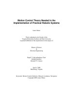
Figure 4.8. Comparison of three control strategies with Jactual = 10*Jassumed (J=10 p.u.)

Chapter 4 The State of Motor Control Academia
42
Conclusion

This chapter covers motor modeling in the state space domain, transformations
from the stationary three-phase reference frame to the rotating reference frame, and
simplified state equation models of DC motors. The sliding mode controller is shown to
have superior disturbance rejection over linear controllers but is impractical due to
chattering. The sliding mode observer with disturbance canceling feedforward is
demonstrated as a method of maintaining superior performance and removing the
chattering problem. The method both improves disturbance rejection with a step

disturbance and improves disturbance rejection and transient times with a sinusoidal
disturbance.
Many other control schemes are possible, and every other advanced control
scheme known to mankind has probably also been applied to motors. All of these
schemes assume some knowledge about the inertia or the torque load. When all
assumptions of knowledge about the system and its load are removed, all these advanced
control schemes reduce to P or PI like schemes. With a plant with only one input and one
output, even sliding mode control reduces to bang-bang control, and bang-bang control is
really P control with a very high gain.
Another example of an advanced linear control scheme that turns out not to help
much is H-infinity control. H-infinity control is the solution to the Problem of
Differential Games, also known as the minimax problem. The problem goes like this:
Assume that all parameter errors and system disturbances will combine in the worse
possible way, the way that causes the most error. Find the set of feedback gains that will
minimize the maximum error. These gains are the H-infinity gains. Because compensator
designers are trying to minimize one thing and maximize another using differential
equations, they are playing a differential game. In the case where there is only one output
and one feedback measurement the H-infinity control reduces to a P controller where a
particular gain is the H-infinity gain. A variation of H-infinity is to add an integrator to
assure zero steady-state error. With only one output and one feedback measurement, the
H-infinity control with integrator reduces to a PI controller.
Chapter 4 The State of Motor Control Academia
43
All linear control techniques suffer from another problem. In PID control the
input to a plant is a weighted sum of output values and the output error goes into a
compensator. In LQR and LQG control the input to the plant is a weighted sum of states
that have been measured or observed from the output of the plant. In the LQR control it is
assumed that some Gaussian noise has been added to the output and a Kalman filter is
used to calculate the states from the output.
In the PID controller proportional, integral, and derivative gains are adjusted until

the plant behaves as desired. In LQR and LQG control the cost of using control, R, and
the cost of error, Q, are adjusted until the plant behaves as desired. Both schemes are hard
to tune analytically because of the inherent non-linearity of the plant and the quality of
the feedback signal. In practice both schemes reduce to experimentally adjusting gains or
costs until the system’s behavior is as close to the desired behavior as possible.
The quality of the feedback signal turns out to be the limiting factor in almost all
control schemes. Increasing gains reach the point where the compensator is no longer
providing more negative feedback but is amplifying the noise in the system. It is common
to see time wasted trying to find a set of gains that compensates for a poor quality
feedback signal. Academia and industry need to place more stress on cleaning up and
filtering feedback signals before attempting to optimize a system by adjusting gains.
Unfortunately high quality and high signal-to-noise ratio feedback devices are expensive
and extra engineering time spent turning knobs is relatively inexpensive, so this situation
is not likely to change soon. It does represent an unexploited market opportunity.
One novel alternative from the usual low-pass and notch-pass filter designs of
undergraduate academia that has potential in the motor control industry is the IIR
predictive filter research led by S. J. Ovaska for smooth elevator control. In [26] Ovaska
et. al. give a good overview of polynomial predictive filters. These filters provide smooth
and delayless feedback when the motor is operating with a smooth profile but have
transient errors when systems have discontinuous acceleration. In [27] Väliviita gives a
method that provides the smooth predicted derivative of a signal that is useful in allowing
high derivative gains. Derivative gains benefit most from this filtering process because
derivation is a noise amplifying process. In [28] Väliviita and Ovaska solve some of the
Chapter 4 The State of Motor Control Academia
44
problems Väliviita had in [27] with the varying DC gain of the filter. With future papers
this method may become more applicable to general purpose motor control.
There are some control schemes that can improve motor control performance with
the same quality feedback signal. One is the use of S-curves and the plotting of velocity
profiles discussed in the last chapter to overcome the problem of the double integrator.

Another is the two degree-of-freedom (DOF) PID controller in which two PID controllers
are used to separately control the characteristics of the transient and the steady state
response. This controller is difficult to tune and is mostly ignored because acceleration
and velocity feedforward gains are already available to control the transient during a
setpoint change. The advantage of 2-DOF PID is its ability to control transients caused by
process disturbances, the problem addressed here. Hiroi [29] [30] [31] has received three
US Patents for 2-DOF controllers and methods of implementing them easily that are in
use by his company but still too complicated for more general use. These controllers have
great potential in industrial control when their use becomes much simpler. The remaining
methods that can achieve better control with the same information are the soft computing
techniques of fuzzy logic and neural networks.

Chapter 5 Soft Computing
45
Chapter 5. Soft Computing

A Novel System and the Proposed Controller

A specific example created by Lewis et. al. in [32] will be used to show how
Fuzzy Logic, a soft computing technique, can improve on the system performance
achievable by either a PID or SMC controller alone. The system is a variation on the
classic inverted pendulum problem. It is an inverted pendulum pinned onto a rotating disk
as shown in Figure 5.1. The pendulum is free to rotate within the plane normal to the disk
at the point of the pin. This plane is itself rotating with the disk.

Figure 5.1. An inverted pendulum of a disk.

Chapter 5 Soft Computing
46
In [32] and [33] Lewis derived the following state equations for the system using

LaGrangian dynamics:
()
()
()
2
22
22
2
4
2
22
2
4
2
222
222
2
4
3
42
31
cos
cossincossin
cos
cossinsin
xlrl
xxlxrxrxmgmrI
x
xrmrI
xxmrgxrlx

x
xx
xx
−
+−+
=
−+
−+
=
=
=
τ
τ
!
!
!
!
(5.1)

Where
θ
and
φ
are the angles of the disk and the pendulum, respectively, as shown in
Figure 5.1 and the state variables are:
φ
θ
φ
θ
!

!
=
=
=
=
4
3
2
1
x
x
x
x
(5.2)

The parameters are:
τ
= torque applied to the disk, the controlling input
r = radius of the disk
l = length to the center of mass of the pendulum
m = mass of the pendulum
g = acceleration due to gravity

A simulation of the system was created using (5.1) and both PID and SMC
controllers were constructed to control the angle of the pendulum to upright. During the
tuning of both controllers the authors became experts on the behavior of the system and
made observations about the system such as the following:
Chapter 5 Soft Computing
47
• The pendulum angle and pendulum speed are the most important states

when controlling the pendulum angle.
• When the pendulum must be righted from large angles and speeds the
SMC performs best
• Once the angles and speeds are small, the PID controller performs best.
The latter observations are because the SMC works by exerting the full available
torque on the disk to rotate it in one direction or the other. This works well for large
errors, but when the error become small the SMC chatters the pendulum around the
upright position. Contrarily, when the errors are small PID control behaves smoothly and
bring the pendulum to a stop in the upright position. When the errors are large the PID
control also provides a large response but creates integrator windup that can cause
unnecessary overshoot and instability.
The solution proposed here is the hybrid control system of Figure 5.2. Here both a
PID and SMC controller calculate a controlling torque based on the error of the pendulum
angle. A Fuzzy Logic controller acts as a soft switch that decides on a weighted average
of the two torques to use as the actual controlling torque based on the angle and velocity
of the pendulum. As noted by the tuning experts, the disk position must be controlled
much more slowly than the pendulum angle. Therefore the pendulum angle in not
controlled to zero, but controlled to bring the disk position to zero with a much slower,
lower gain disk position loop wrapped around it. This outer loop is a PID controller and
is of little interest to object of this example, a fuzzy logic approach to getting the best
qualities of two different controllers. The outer loop is included for a practical reasons: a
spinning disk with an erect pendulum is dizzying to watch, hard to graph, and requires
the pendulum angle measurement device to be connected wirelessly or with a slip ring.
Chapter 5 Soft Computing
48
VELOCITY
POSITION
WEIGHT
SUM
SUM

PID
SMC
PID
INV E RTE D
PENDULUM
FUZZY CONTROLLER
0
DESIRED
POSITION
ANGLE


Figure 5.2.
Inverted Pendulum on a disk and its control system.


The Fuzzy Controller

Experts tuning the system can come up with a set of linguistic rules describing
when it is best to use which controller based on the pendulum angle and velocity. These
rules can be put in an IF-THEN form using the linguistic variables Small, Medium, and
Large to describe pendulum angle and velocity and the appropriate weight of the SMC
controllers output. Some of these rules are:
• IF the Angle is Small AND the Velocity is Small THEN the SMC weight should be Small.
• IF the Angle is Medium AND the Velocity is Medium THEN the SMC weight should be Small.
• IF the Angle is Large AND the Velocity is Large THEN the SMC weight should be Large.
With two measured states and three linguistic variables describing each there are
nine such possible rules. One of the advantage of Fuzzy Logic controllers is that it is not
necessary to have every possible linguistic rule. This is especially advantageous as the
number of rules increases. This and other variation and complexities of a Fuzzy Logic

controller are given a thorough discussion by Jang et. al. [34]. The system here has only