Motion Control Theory Needed In The Implementation Of Practical Robotic Systems 2 Part 10 pptx
Bạn đang xem bản rút gọn của tài liệu. Xem và tải ngay bản đầy đủ của tài liệu tại đây (66.47 KB, 8 trang )
Chapter 7 A Conclusion with an Example
65
vehicles utilize regenerative braking. When the vehicle is stopping the kinetic energy of
vehicle motion is returned to the chemical potential energy of a more fully charged
battery. Demanding consumers and the need to reduce customer support costs have
probably resulted in a well developed, debugged, and documented system. Manufacturing
and system construction have been standardized to the point where an entire bicycle can
be purchased assembled or the power system can be purchased separately as a kit.
ZAP products are a good example of what it takes to turn a working research lab
or academic prototype into a commercial product. They have avoided a premature entry
into the full size electric passenger vehicle market that is only now becoming mature
enough to flourish. They have left the most complex control tasks usually assigned to
electric vehicles, steering and navigation, to the system that still does it best: the human
operator.
Chapter 8 Introduction to Navigation Systems
66
Part II. Automated Navigation
Chapter 8. Introduction to Navigation Systems
Battery
Battery
Motor
Control
Motors
Topics Covered Here
Navigation
Control
Cameras
Vision
System
Other
Sensors
Manual
Control
WHEELS
Figure 8.1. A typical autonomous vehicle system showing the parts discussed here.
When many people think about electric vehicles they think about autonomous
electric vehicles. Autonomous vehicle, electric vehicle, and hybrid electric vehicle
technologies are likely to converge as these technologies mature. The motor control
Chapter 8 Introduction to Navigation Systems
67
aspect of designing electric vehicles was the subject of Part I. The object of Part II is
taking the human out of the loop and getting vehicles to drive themselves.
All robots need some sort of sensors to measure the world around them. Other
than cameras the staples of robotics sensors are ultrasonics, tactile sensors, and infrared
sensors. Ultrasonic sensors are used as range finders, emitting a ping of high frequency
sound and measuring the time-of-flight until the echo. Tactile sensors are bumpers with
switches that only provide information about when a robot has hit something. Infrared
sensors can be used as rangefinders or as motion detectors. All these sensors are not only
economical but relatively easy to process they provide only a single point of
information and only so much can be done with that single point. Successful designs
using these sensors quickly move to designs using arrays of sensors or multiple
measurements over time.
Cameras are a huge step up from these other sensors because the two-dimensional
array of information they provide is a flood of data compared to the single drops of
information provided by other devices. Quality cameras, interfaces, video capture
hardware, and computers are required to quickly and effectively process entire images. In
[43] Mentz provides a good example of image processing hardware selection. In a
general sense an image can be a 2D array from sonar, radar, camera, or other data and the
techniques that apply to each are captivatingly similar.
Three recent or emergent technological advances are underutilized in the
development of new computer vision hardware. The first two address the problem of
dynamic range when using cameras outdoors. Outdoor images often have single points
where direct sunlight is reflected into the camera. When this happens the Charged
Coupler Devices used to detect light in conventional CCD cameras will completely fill
with charge and overflow, or bloom, into adjacent cells. CCD cameras also have very
poor rejection of infrared light. This causes hot objects, usually the dark objects that are
not reflecting sunlight, to emit enough infrared radiation to alter a pixel’s correct
intensity. The result is that nothing in the image looks good and outdoor images are
almost always grainy and washed out compared to images captured in a lab.
Chapter 8 Introduction to Navigation Systems
68
The technological advance that is doing the most to solve the problem of poor
dynamic range is the CMOS camera. These cameras use a photodiode or photogate and
active transistor amplifier at every pixel site to create a camera chip out of conventional
fabrication processes and virtually eliminate the problems associated with CCD’s. A few
major semiconductor manufacturers are making CMOS cameras, but the industry leader
is Photobit [44]. They have a CMOS camera right for every need, robotics or otherwise,
and are poised to become the ubiquitous standard in camera chips.
The next new technology is a new thermoelectric material by Chung et. al. [45]
that exploits the thermoelectric cooling effect. When current flows through a PN junction
both electrons and holes move away from the interface and take heat with them. The new
material exploits this phenomenon better to produce solid state refrigerators on a card that
can be driven to 50°C below ambient. This is useful because dark currents, falsely
detected light caused by the electron drift in all materials over absolute zero, plague CCD
chips. CCD chips are also heated by their own high power consumption. A thermoelectric
heat sink could keep these chips cool enough to significantly improve performance.
Thermoelectric cooling will also benefit any infrared camera technology because this
band is so sensitive to heat.
Finally, recent advances in embedded computing performance offer the
opportunity for significant increases in real-time image filtering and color space
transformation. The TI C64x DSP [46] offers 8800 MIPS of performance, or over 954
instructions per pixel for a 30 frame per second VGA signal. This has the potential to
move many major image processing tasks into real-time hardware and make them
invisible to higher level software. A discussion of image processing techniques will
generate an appreciation for the need for brawny vision processing computer power.
Chapter 9 Image Processing Techniques
69
Chapter 9. Image Processing Techniques
Image processing techniques are as varied as their possible application but the
general steps of filter, segment, and measure are common. The steps required in a typical
electric vehicle application will be reviewed here as an example. The vehicle may be on a
paved or unpaved roadway but is attempting to navigate along a path that usually
contains a solid or striped line on one or both sides. There are arbitrary obstacles along
the path. The vehicle is equipped with a single color forward-looking camera that must
detect the line segments on either side of the path and any obstacles.
The first step is to acquire an image from the camera and measure the dynamic
range and contrast of each color channel. This information is used to adjust the gain and
exposure time of the next frame. The camera parameters that need to be automatically
controllable, especially focus and zoom, greatly affect the cost of the entire system.
The next step is to stretch the image across the full dynamic range of the
colorspace to create as much distinction as possible for future operations. In the process
an attempt may also be made to correct for inconsistent shading, speculars, noise, and
blooming. After this the image will be converted from the camera’s native colorspace,
usually Red-Green-Blue, to the Hue-Saturation-Intensity colorspace. The hue describes a
color pixel’s angle from red around the color wheel, and is mostly invariant with changes
in lighting conditions. The hue is the only component of the new color space that will be
kept for this example. Saturation describes how vivid a color is and is difficult to use in
image processing; it is the first piece of information lost in most image compression
schemes and the first piece of information completely corrupted by sunlight and infrared.
The best use of saturation may be in textured surfaces where the saturation changes with
the viewing angle and shape-from-saturation transforms may be possible. Intensity is the
black-and-white channel of the image and is all that is available on monochrome
cameras. It may be wise to repeat an image processing algorithm with just the hue and
just the intensity and compare the results.
After transforming the image and keeping the hue channel, a series of linear
convolutions are usually applied to clean up noise in the image. The main complication
Chapter 9 Image Processing Techniques
70
arises when there is a need to apply non-linear filters to an image. For example, the
Adaptive Wiener 2 filter [47] is a non-linear blurring filter that blurs areas with edges less
than areas with low variance in an attempt to remove noise without blurring the edges of
objects. Color space transformation are generally non-linear and the order of all the non-
linear operations can have a tremendous effect on the resulting image.
A threshold or a series of morphological operators may be applied to further
remove spurious features from the image. The image is then segmented into objects of
interest through either connected component labeling or a clustering algorithm. A popular
variation of these classic segmenting methods in the region-of-interest or ROI. When
using ROI’s a finite number of windows from the original image are kept and the entire
image processing sequence is only performed on these windows. After the process is
complete the center of the object in each ROI is found and the coordinates of the ROI are
adjust in an attempt to get the object closer to the center of the ROI on the next image. If
there is no object in the ROI sophisticated searching algorithms may be employed to
move the ROI in search of an object. This technique was originally used because image
processing hardware did not have the power to perform the desired operations on the
entire image fast enough. It is still in use because it turns out to be an excellent method of
tracking objects from one frame to the next.
The final task is to extract some useful information about the components that
have been separated from the image. This system assumes all components are either long
skinny line segments or blob-like obstacles. Sophisticated pattern matching techniques
including Bayesian classifiers and neural networks may be used to compare a segment to
a library of known objects. The optics of the camera and geometry of its location on the
vehicle will be used to carry out a ground plane transform, a transform that determines
the coordinates of a pixel in an image by assuming that the object lies on a level ground
plane. The vision system then passes along information useful to the navigation system: a
list of line segments and obstacles and their coordinates in the ground plane.
Chapter 10 A Novel Navigation Technique
71
Chapter 10. A Novel Navigation Technique
Every autonomous vehicle navigation strategy will undergo many revisions and
incremental improvements before it works reliably. The result of evolving a navigation
strategy for the example of the previous chapter with line segment and obstacle data is
presented here. All obstacles will be represented by the potential field shown in Figure
10.1. This scheme has been named Mexican Hat Navigation because of Figure 10.1’s
shape.
Figure 10.1. The Mexican Hat. A potential field that will be used to represent an obstacle.
This shape is known as the 2D Laplacian of Gaussian and is a statistical
distribution that has been commonly used in edge detection ever since vision pioneer
David Marr [48] suggested that it is the edge detection convolution carried out by the
human retina. The Laplacian of Gaussian is a well established function that will be used
in a novel way. In the human eye a bright dotted line activates the retina with the activity
map of Figure 10.1. The troughs on each side of the dotted line combine to form two
valleys of dark outlining a mountain range of light peaks which are then perceived as a
single line. This function’s penchant for well behaved superpositioning makes it an ideal
basis for an entire navigation strategy. The trough around the peak has been placed at a
Chapter 10 A Novel Navigation Technique
72
distance that corresponds to a safe distance for a vehicle to pass an obstacle based on the
width of the vehicle. When multiple obstacles are present their fields overlap to create
troughs in places through which the vehicle can safely navigate.
The world chosen for this example contains only two objects, obstacles and line
segments. All line segments will be represented by the potential field shown in Figure
10.2. This Figure is known as the Shark Fin. It has a Laplacian of Gaussian distribution
perpendicular to the line segment and a Gaussian distribution parallel to the line segment.
Figure 10.2. The Shark Fin. A potential field that will be used to represent a line segment.
All the line segments and obstacles detected by the vision system and any
obstacles detected by other systems are mapped together onto the empty grid in Figure
10.3. At each obstacle location a Mexican Hat mask is added to the grid. For each line
segment a Shark Fin must be translated and rotated before it is added to the grid. The
result of all these superpositioned masks is the potential field of Figure 10.4.
The vehicle, which starts at the bottom center of the map, navigates by driving
forward down the potential alley of least resistance. This path is shown on the field in
Figure 10.5 and again on the original map in Figure 10.6.