Derivatives Demystified A Step-by-Step Guide to Forwards, Futures, Swaps and Options phần 4 potx

7
Equity and Credit Default Swaps
EQUITY SWAPS
An equity swap is the over-the-counter alternative to equity index and single stock futures. It
is an agreement between two parties:
r
to exchange payments at regular intervals;
r
over an agreed period of time;
r
where at least one of the payment legs depends on the value of a share, a basket of shares or
a stockmarket index.
In a total return deal a payment is also made which reflects the dividends on the share or
basket or index. A typical equity swap application occurs when a company owns a block of
shares in another firm (this is sometimes known as a corporate cross-holding) which it would
like to ‘monetize’, i.e. to sell for cash. However, the company wishes to retain the economic
exposure to changes in the value of the shares for some time period. The company sells the
shares and enters into an equity swap in which it receives the return on the shares paid in cash
on a periodic basis.
MONETIZING CORPORATE CROSS-HOLDINGS
To illustrate the idea, suppose that a company owns a block of 100 million shares in another
firm. The shares are worth €1 each, with a total value of €100 million. It sells the shares to
a bank and at the same time enters into a one-year equity swap. The notional principal is set
at the outset at €100 million, although this will be reset later depending on what happens to
the value of the shares. In the swap the bank pays the company the total return on the block
of shares (capital gains or losses plus dividends) on a quarterly basis. In return, the company
pays Euribor on a quarterly basis. Euribor is a key reference rate for short-term lending in
euros, calculated by the Brussels-based European Banking Federation (FBE). The quarterly
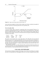
payments are illustrated in Figure 7.1.
There will be four payments on the swap, the first being due three months after the start
date. The Euribor rate for that first payment is fixed at the start of the contract. Let us suppose

that it is set at 4% p.a. or 1% for the quarter, so that the company will owe the bank €1 million
on the interest rate leg of the swap. Suppose also that on that first payment date the shares
are worth €102 million. The bank then owes the company €2 million for the increase in the
value of the shares from the starting level of €100 million. We will assume that there are no
dividends that quarter. Then all the payments are as follows:
r
The company owes an interest payment of €1 million.
r
The bank owes €2 million for the increase in the value of the shares.
r
The payments are netted out and the bank pays the company €1 million.
60 Derivatives Demystified
COMPANY BANK
Total return on shares
Three-month Euribor
Figure 7.1 Equity swap payment legs
The notional principal amount and the Euribor rate are now reset to help to calculate the cash
flows due on the next quarterly payment date (six months after the start date of the swap). The
notional principal value is reset to €102 million, the current value of the shares. For simplicity
we will assume that the Euribor rate is unchanged at 4% p.a. and that no dividends are paid in
the next quarter. Suppose that on the second payment date the shares are worth €99 million.
The payments due on the swap for that quarter are calculated as follows:
r
The company owes 1% of €102 million in interest which is €1.02 million.
r
The company also owes €3 million for the fall in the value of the shares from a level of
€102 million.
r
The company pays the bank a total of €4.02 million.
If the shares increase in value during a quarter, the bank pays the company for the increase, but

if the shares fall in value the company pays the bank. This replicates the economic exposure
the company would have if it actually retained the shares. It is also possible to fix the notional
on an equity swap throughout the life of the contract. A floating or resetting notional swap
replicates an exposure to a fixed number of shares. A fixed notional equity swap replicates an
exposure to a fixed value of shares, such that if the share price rose or fell the investor would
sell or buy shares to maintain a constant allocation.
OTHER APPLICATIONS OF EQUITY SWAPS
Equity swaps are extremely versatile tools and have many applications for companies, banks
and institutional investors. Because they are over-the-counter deals negotiated directly between
the two parties, they can be tailored or customized to suit the needs of clients. A dealer will
normally agree to pay the return on almost any basket of shares, provided some means can be
found to hedge or at least to mitigate the risks on the transaction.
This can be useful, for example, for an investor who wishes to gain exposure to a basket
of foreign shares but faces certain restrictions on ownership. A swap dealer will agree to pay
the return on the shares (positive and negative) every month or every three months for a fixed
period of time. In return, the investor will pay a floating or fixed rate of interest applied to the
notional principal. The deal can be structured such that all the payments are made in a familiar
currency such as the US dollar or the euro.
In this kind of case, it is possible that if the investor actually purchased the underlying shares
then, as a foreigner, he or she would have to pay tax on the dividend income. If this is the case,
the investor can enter into an equity swap transaction with a dealer who is not subject to the tax
or can reclaim it. The dealer borrows money to buy the shares, and in the swap transaction the
Equity and Credit Default Swaps 61
INVESTOR BANK
Total return on shares in $
$ LIBOR + 0.3%
PURCHASE
SHARES
Total return on shares in local currency
Figure 7.2 Investor paid total return on a swap including gross dividends

dealer pays the total return on the shares to the investor, including gross dividends. In return
the investor pays a funding rate which the dealer uses in part to service the loan and in part
to make a profit on the transaction. The series of transactions involved in this type of deal is
illustrated in Figure 7.2. In this swap the bank pays the total return on the shares to the investor
in US dollars. The investor pays US dollar LIBOR plus 30 basis points.
The bank borrows money to buy the shares and uses the dollar LIBOR payment from the
swap to help to pay the interest on the loan; assuming that it can borrow at LIBOR it will
make 30 basis points per annum on the deal. It will need this, not just to make a profit, but also
because its hedge is unlikely to be perfect and it will have to manage the risks. For example,
although the bank has agreed to pay over the return on a specific basket of shares it may decide
to hedge by buying a subset of shares in the basket in order to save on transaction costs. It will
also have to manage the currency translation since it is making payments on the swap in US
dollars whereas the returns on the underlying shares will be achieved in local currency.
By entering into an equity swap, it is just as easy for a client to take a ‘short’ position in a
share or a basket of shares as it is to take a long position. The client agrees to pay over to the
swap dealer any changes (positive and negative) in the value of a share. If the share price falls
the client will receive payments from the swap dealer; if it rises the client will have to make
payments to the dealer. Economically, this is the equivalent of a short position.
Of course it is also possible to take long and short positions in shares by trading equity
index and single stock futures (see Chapter 5). One drawback of futures is that there is a daily
margin system in operation, which may be inconvenient. With an equity swap there are a set
number of payments, made weekly, monthly or quarterly. Swaps can also be customized to
meet the needs of clients. On the other hand, futures are guaranteed by the clearing house,
whereas swaps are over-the-counter transactions and, as such, carry counterparty default risk.
62 Derivatives Demystified
EQUITY INDEX SWAPS
In a standard equity index swap contract one party agrees to make periodic payments based on
the change (positive or negative) in the value of an equity index such as the S&P 500, the DAX,
the Nikkei 225, the CAC 40 or the FT-SE 100. In return it receives a fixed or a floating rate
of interest applied to the notional principal. The swap can be structured such that the notional

principal remains constant over the life of the deal, or varies according to the changing level
of the index.
The term sheet for a typical equity index swap transaction is set out in Table 7.1. The deal is
also illustrated in Figure 7.3 (the  sign simply means ‘change’). The swap dealer has agreed
to pay the total return on the FT-SE on a quarterly basis, including a payment representing the
dividend yield on the index. In return the dealer receives three-month sterling LIBOR plus 25
basis points applied to the notional principal. The notional is fixed at £100 million, the LIBOR
rate and dividend yield for thefirst payment have been set at 3.75% p.a. and 3% p.a. respectively,
and the starting index level is fixed at 5000 points. This is based on the level of the cash FT-SE
100 index when the deal is agreed.
The first payment on the swap is due three months after the start date. We will assume that
the FT-SE 100 index is trading at 5100 at that point, which is a rise of 2% from the starting
level of 5000. The payments due on the swap are then calculated as follows:
r
The dealer pays 2% of £100 million for the rise in the index, i.e. £2 million.
r
The dividend yield was set at 3% p.a., which is 0.75% for the quarter. Applied to the notional
of £100 million, this means that the dealer pays £0.75 million.
r
The LIBOR rate was fixed at 3.75% p.a. Including the spread, the client owes 1% of £100
million for the quarter, i.e. £1 million.
r
Payments are netted out and the dealer pays £1.75 million to the client.
Table 7.1 Equity index swap on the FT-SE 100
Client receives: Change in the value of the FT-SE 100 index plus the dividend yield
on the index
Dealer receives: Three-month sterling LIBOR + 0.25%
Payments for both legs: Quarterly
Start date: Today
Maturity: In one year

Notional principal:
£100 million fixed
First LIBOR setting: 3.75% p.a.
First dividend yield setting: 3% p.a.
Start FT-SE level: 5000
CLIENT
SWAP
DEALER
Three-month £ LIBOR + 0.25% p.a.
∆ FT-SE 100 + dividend yield
Figure 7.3 Equity swap payment legs
Equity and Credit Default Swaps 63
The key variables are reset to help to establish the second payment on the swap, which is due
after a further three months. The variables are as follows:
r
the FT-SE 100 index level, which in this case will be reset at 5100
r
the interest rate, which is re-fixed according to three-month sterling BBA LIBOR
r
the dividend yield on the FT-SE 100 index.
Since the swap has a maturity of one year with quarterly payments, this means that there
will be a total of four payments, all calculated in the manner illustrated above. At maturity
the final payment takes place and the swap expires. The swap enables the client to achieve
a diversified exposure to the UK stock market, without having to physically buy the shares,
which could incur significant spreads and other transaction costs. The client pays LIBOR plus
a set spread. In fact the interest rate could easily be fixed by adding an interest rate swap to the
package.
Hedging equity swaps
In the above example, the dealer pays the total return on the FT-SE 100 index to the client.
If the index rises the dealer pays the client for that increase, but if the market falls the client

pays the dealer. In effect, the dealer has a short position in the FT-SE 100 index. The dealer
can hedge the risk if he or she buys FT-SE 100 index futures (see Chapter 5). This establishes
a long position in the market so that profits and losses on the futures contracts will offset those
on the swap. The dealer would, however, have to buy futures contracts that match the payment
dates on the swap, and there is the risk that the contracts might be expensive, i.e. trading above
their fair or theoretical value.
As an alternative, the dealer could borrow money and buy a basket of shares designed to
track the FT-SE 100 index, and use the LIBOR-related receipts on the swap to service the
interest payments on the loan. The hedge is illustrated in Figure 7.4. The dealer simply pays
CLIENT
SWAP
DEALER
∆ FT-SE 100 + dividend yield
BUY
SHARES
∆ FT-SE 100 + dividends
Three-month £ LIBOR + 0.25%
Figure 7.4 Equity swap hedged in the cash market
64 Derivatives Demystified
BUYER OF
PROTECTION
SELLER OF
PROTECTION
Premium
× basis points p.a.
Payment contingent on credit event
Figure 7.5 Credit default swap
away the returns on the shares to the client in the equity swap transaction. Assuming the loan
can be funded at exactly LIBOR, then the dealer has covered the equity exposure and has
made 25 basis points on the set of transactions. The dealer also has to consider counterparty

or default risk on the swap; in practice, the client may be asked for collateral when the deal is
agreed to cover this risk.
CREDIT DEFAULT SWAPS
Generally, a credit derivative is a contract whose payout depends on the creditworthiness
of some organization such as a multinational corporation. Specifically, a credit default swap
(CDS) is a form of insurance against default on a loan or a bond. There are two parties to a
deal:
r
The buyer of protection.
r
The seller of protection.
The asset that is to be protected is known as the referenced asset. It can be a loan or a bond
or a set of such obligations. The borrower or issuer of the bond is called the referenced credit
or entity. In the standard type of deal the buyer of protection pays a periodic premium to the
seller of so many basis points per annum applied to the par value of the referenced asset (this
can also be made in a single up-front payment). If, during the life of the swap, any one of a
number of specified credit events occurs then the seller of protection has to take delivery of
the referenced asset and pay a set amount of money to the buyer of protection (normally the
par value of the asset). The swap can also be set up such that if a credit event occurs the buyer
of protection retains the asset but is paid cash in compensation. The basic deal is illustrated in
Figure 7.5.
A range of credit events affecting the referenced credit can be stipulated that will trigger
the contingent payment by the seller of protection. This can include items such as bankruptcy,
insolvency, failure to meet a payment obligation when due, a credit ratings downgrade below
a certain threshold. The payout on a basket CDS is based on a basket of assets with different
issuers. In a first-to-default deal the credit event that triggers payment depends on the first of
the referenced assets in the basket that defaults. Buyers of protection in credit default swaps
include commercial banks who wish to reduce their exposure to credit risk on their loan books,
and investing institutions seeking to hedge against the risk of default on a bond or a portfolio
of bonds. Sellers of protection include banks and insurance companies who earn premium in

return for insuring against default.
Most deals are structured such that if a credit event occurs the buyer of protection sells
the referenced asset to the seller of protection at a set price. However, some assets cannot be
Equity and Credit Default Swaps 65
Table 7.2 Users of credit derivatives 2003
Types of institution Protection buyer (%) Protection seller (%)
Banks 52 39
Securities houses 21 12
Hedge funds 12 21
Corporates 4 16
Monoline/re-insurers 3 5
Insurance companies 3 3
Mutual funds 2 2
Pension funds 1 2
Governments/agencies 2 0
Source: British Bankers’ Association, Lehman Brothers. Quoted in Financial News
transferred for legal reasons, in which case the buyer of protection is given the right to substitute
a similar asset that can be transferred. If the deal is structured such that the protection buyer
actually retains the asset but is compensated in cash for the fall in its value, then some means
has to be found to establish the value of the asset after a credit event occurs. This is often
estimated through a series of dealer polls, since it is not likely that the asset would be actively
traded in such circumstances.
To give some idea of the size of the market, the International Swaps and Derivatives Asso-
ciation (ISDA) estimated that the notional principal amount outstanding on credit derivatives
generally at mid-year 2003 was $2.69 trillion, compared to $2.79 trillion on equity derivatives.
(These values are adjusted for double-counting.) ISDA provides important services for the
market, including standard documentation for credit default swaps. Table 7.2 shows the users
of credit derivatives in 2003 and the proportions that bought and sold protection.
Credit default swap premium
The periodic premium paid on a credit default swap is related to, but not normally exactly the

same as, the credit spread on the referenced asset. The credit spread is the additional return
that investors can currently earn on that asset above the return available on assets that are free
of default risk – in effect, Treasury bonds.
For example, suppose that a five-year corporate bond pays a return of 5% p.a. and the return
on five-year Treasuries is only 4% p.a. Then the bond’s credit spread is 1% p.a. or 100 basis
points. The size of the spread depends to a large extent on the rating of the bond, which measures
the probability of default. It also depends on other factors such as the expected recovery rate if
it defaults – the percentage of the par value the investors can hope to recover from the issuer.
The seller of protection in a credit default swap assumes the credit risk on the referenced asset
and should therefore be paid a premium that reflects the level of default risk on that asset – i.e.
one that is related in some way to its credit spread.
Suppose that an insurance company has invested in risk-free Treasury bonds. The returns
are safe but not very exciting. It decides to enter into a credit default swap in which it receives
a premium in return for providing default protection against a referenced asset. The position
of the insurance company is illustrated in Figure 7.6.
By entering into the swap the insurance company has moved from a risk-free investment to
a situation that involves credit or default risk. To an extent this replicates the sort of position
66 Derivatives Demystified
BUYER OF
PROTECTION
INSURANCE
COMPANY
Premium X basis points p.a.
Payment contingent on credit event
TREASURY
BONDS
Risk-free return
REFERENCED
ASSET
Risk-free return +

spread
Figure 7.6 Treasury bonds plus credit default swap
it would be in if it sold the Treasuries and bought the referenced asset itself. The premium
received from the buyer of protection in the swap should therefore be related to the additional
return over the risk-free rate (the credit spread) available on the referenced asset. In practice,
credit default swap premiums are not usually exactly the same as the spread over Treasuries on
the referenced asset for a variety of reasons. The spread is affected by the liquidity of the asset
as well as its default risk. As another complicating factor, the two parties in a credit default
swap also acquire a credit exposure to each other.
There are a number of ways in which the premiums on credit default swaps are established.
One is by modelling the probability of default on the referenced asset, based on the credit
spread and/or the historical behaviour of assets of that credit quality. The ratings agencies
publish historical default rates and recovery rates on different classes of assets with different
credit ratings. They also publish so-called transition matrices which provide historical data on
the occurrence of ratings downgrades on assets with different credit qualities.
When calculating the CDS premium it is necessary to take into account the expected recovery
rate on the referenced asset – that is, the percentage of its par value that can be recovered in
the event of default. This will depend on factors such as the seniority of the asset and whether
it is secured on collateral such as property.
CHAPTER SUMMARY
An equity swap is an agreement between two parties to exchange cash flows on regular future
dates where at least one of the payment legs depends on the value of a share or a portfolio
of shares. The notional principal on a deal can be fixed or floating. Traders and investors can
replicate long and short positions in shares by receiving or paying the change in the value of
the underlying in an equity swap. In a total return deal, dividends are also paid. In an equity
index swap one of the payment legs is based on a stockmarket index such as the S&P 500 or
the FT-SE 100. A deal can be hedged by trading index futures or by buying or shorting the
underlying shares.
Equity and Credit Default Swaps 67
In a credit default swap the buyer of protection pays a premium to the seller of protection.

In return he or she receives a contingent payment depending on whether one of a number of
credit events occurs during the life of the agreement. Credit events can include default or ratings
downgrades or financial restructurings. The premium on a credit default swap depends on the
probability that a credit event will occur and also on any money that can be recovered on the
asset or assets being protected. Buyers of protection include fund managers and commercial
banks seeking to reduce the level of credit risk on portfolios of bonds or loans. Sellers of
protection include dealers in banks, and insurance companies who are trying to enhance the
returns on their investments by earning premium.

8
Fundamentals of Options
INTRODUCTION
In Chapter 1 we saw that options on commodities such as rice, oil and grain have been in
existence for many years. Options on financial assets are more recent although activity has
expanded rapidly since the introduction of listed contracts on exchanges such as the Chicago
Board Options Exchange (CBOE), LIFFE and Eurex. The buyer of a European-style option
contract has the right but not the obligation:
r
to buy (call option) or sell (put option) an agreed amount of a specified asset, called the
underlying;
r
at a specified price, called the exercise or strike price;
r
on a future date, called the expiry or expiration date.
European options can only be exercised at expiry, whereas American-style contracts can be
exercised on any business day up to and including expiry. These labels are purely historical.
The majority of exchange-traded options around the world are American-style, modelled on
the contracts first traded on exchanges in the USA. Over-the-counter (OTC) options are often
European, because the buyers do not wish to pay extra premium for the ability to exercise
before expiry. An American call on a dividend-paying share will be more expensive than a

European call, since there are occasions when it is beneficial to exercise the contract early and
receive the forthcoming dividend on the share. A Bermudan option is a half-way house. It can
be exercised on a set number of days before expiry, such as one day per week.
Unlike a forward, an option contract has built-in flexibility because the holder is not obliged
to exercise or take up the option. For this privilege the buyer of an option has to pay an initial
premium to the seller (also known as the writer) of the contract. As we will see in Chapter 13,
the premium is determined by calculating the expected payout, and a key input to establishing
this value is the volatility of the price of the underlying asset. The more volatile the underlying
asset, all other things being equal, the greater the expected payout from an option on that asset,
and the greater the premium charged by the writer.
Consider the example of a one-year European call on a share struck at $100. The holder of
the option has the right but not the obligation to purchase the share for $100 after one year.
If the price of the share is highly volatile this increases the chance that it will be substantially
above the strike at expiry. The greater the value of the underlying at expiry, the greater the
profit achieved by the owner of the call. Of course, a high level of volatility also increases
the chance that the share price at expiry will be below the $100 strike of the call. However
the holder of the option is not obliged to exercise the contract. The loss is limited to the initial
premium paid.
Exchange-traded options are largely standardized but their performance is guaranteed by the
clearing house associated with the options exchange. OTC options are agreed directly between
two counterparties, one of which is normally a specialist dealer at a bank or securities firm. As
70 Derivatives Demystified
Table 8.1 Bought call option contract
Type of option: Long call
Underlying share: XYZ
Spot share price: $100
Number of shares in the contract: 100
Exercise price: $100 per share
Exercise style: American
Expiry: 1 year

Premium: $10 per share
a result, the terms of OTC contracts can be tailored to meet the needs of clients. For example,
the strike price or the time to expiry can be adjusted; or the contract can be based on a basket
or portfolio of shares rather than a single asset. The contract can also be designed such that
profits and losses are settled in cash rather than through the physical delivery of the underlying
asset. This is an advantage for clients who do not wish to go through the inconvenience and
expense of an actual delivery process.
CALL OPTION: INTRINSIC AND TIME VALUE
A call option is the right but not the obligation to buy a commodity or a financial asset at a
fixed strike or exercise price. Table 8.1 gives details of an equity call option contract purchased
by a trader. The option is American-style, so it can be exercised on any business day up to and
including expiry, in one year’s time. The underlying share is trading at $100 in the cash or spot
market and the exercise price of the call is also $100. The premium charged by the writer of
the contract is $10 per share or $1000 on 100 shares.
The holder of the call has the right to purchase each share for $100. The intrinsic value
of an option is defined as any money that can be realized through immediately exercising the
contract. In this case the share is trading at $100 in the cash market and the strike is also $100, so
the holder cannot release any value by immediate exercise. The option has zero intrinsic value.
Since the strike price is exactly the same as the spot price, the call is said to be at-the-money.
Imagine, however, that some time after the option is purchased the spot price of the share
jumps to $120. The option is now in-the-money since the owner has the right to buy a share
for $100 that is worth $120. The option contract now has $20 intrinsic value per share.
Note that this is not the net profit the holder would achieve by actually exercising the call.
To establish this value the initial $10 premium has to be deducted from the intrinsic value.
Table 8.2 calculates the option’s intrinsic value if the spot price of the share moves to a range
Table 8.2 Intrinsic value of $100 strike call for a range of
spot prices
New share price Intrinsic value now Option is now . . .
$80 $0 Out-of-the-money
$90 $0 Out-of-the-money

$100 $0 At-the-money
$110 $10 In-the-money
$120 $20 In-the-money
Fundamentals of Options 71
of different possible levels. Notice that intrinsic value is never negative because the owner of
an option is never obliged to exercise an out-of-the-money contract.
More formally, the intrinsic value of an American-style call option can be defined as the
spot price of the underlying asset minus the strike, or zero, whichever is the greater of the
two. This definition is commonly also applied to European options, although the profit from
exercise can only be realized at expiry.
Any money paid for an option in addition to its intrinsic value is called time value.Inthe
contract shown in Table 8.1, the buyer pays $10 per share in premium, even though the option
has no intrinsic value at all. The $10 consists of time value, and the buyer is obliged to pay this
money because there is some chance or probability that the share price might rise above the
strike before expiry. This possibility provides profit opportunities for the buyer of the contract
and serious risks for the writer. If the contract is exercised the writer is obliged to deliver a
share at a fixed price of $100, whatever its value in the market happens to be at that point in
time. The buyer of the call has to pay for that chance or opportunity and the writer has to be
compensated for that very considerable risk. The two components – intrinsic and time value –
together make up the total premium paid for an option.
Option premium = Intrinsic value + Time value
The expression time value derives from the fact that normally, all other things being equal,
a longer-dated option has more time value than a shorter-dated contract. The probability of
a share price doubling in the course of a year is much greater than over the course of a day.
This increases the potential payout to the buyer of a call on the share. It also increases the
potential losses to the writer, who has to charge a higher premium in compensation. Talk of
‘time value’ can be a little misleading, however, since time to expiry is not the only factor that
determines how much a buyer has to pay for an option over and above its intrinsic value. It
is also determined by factors such as the volatility of the underlying, and the general level of
interest rates in the market. We will return to this issue in Chapter 13.

Long call expiry payoff
If an option is at- or out-of-the-money at expiry it has zero intrinsic value. The contract will
simply not be exercised and will be worthless. On the other hand, if the option is in-the-money
it will have positive intrinsic value. This is calculated as the difference between the share price
and the strike price. At expiry an option has zero time value, since the outcome of the contract
is no longer in question.
To illustrate these effects, we return to the bought or ‘long’ call option contract discussed in
the previous sections. The strike is $100 and premium paid is $10 per share. Table 8.3 shows
the intrinsic value for a range of different possible share prices at expiry. The break-even point
occurs when the underlying is trading at $110. The owner of the call can realize $10 intrinsic
value by exercising the contract, by purchasing a share for $100 that is worth $110. This
exactly offsets the initial premium, and the net profit and loss per share is zero. (This ignores
any transaction and funding costs.)
The results from Table 8.3 are presented graphically in Figure 8.1, which shows the net profit
and loss on the option contract for a range of possible share prices between $50 and $150. The
maximum loss to the buyer of the call is $10 per share. The maximum profit is unlimited since
the share price (in theory) could rise to any level.
72 Derivatives Demystified
Table 8.3 $100 strike call: intrinsic value and net P&L at
expiry per share
Share price at expiry Call intrinsic value Net profit and loss
50 0 −10
60 0 −10
70 0 −10
80 0 −10
90 0 −10
100 0 −10
110 10 0
120 20 10
130 30 20

140 40 30
150 50 40
-50
-30
-10
10
30
50
50 70 90 110 130 150
Share price at expiry
Net P&L per share
Figure 8.1 Profit and loss per share on long $100 strike call at expiry
Short call expiry payoff
In the jargon of the market, the buyer of an option contract has limited downside (potential
losses) but unlimited upside (potential profit). Like an insurance policy, the most money that
can ever be lost is the initial premium that was paid. Also, if the option is exchange-traded it
can easily be sold back before expiry, recouping at least some of that initial outlay.
However the position of the seller or writer of a call option is very different. Figure 8.2
illustrates the payoff profile at expiry for the writer of the call option explored in the previous
sections. The maximum profit is the initial premium collected. If the share price is trading
above the strike at expiry then the option will be exercised at a profit to the holder and a loss to
the writer. For example, suppose the share price is $150. Then the writer will have to deliver
a share at a fixed price of $100 which costs $150 to buy in the spot market, so losing $50 on
exercise. From this is deducted the initial premium received of $10, leaving a $40 loss per
share on the deal (ignoring funding and transaction costs).
Fundamentals of Options 73
Table 8.4 Bought put option contract
Type of option: Long put
Underlying share: XYZ
Spot share price: $100

Number of shares: 100
Exercise price per share: $100
Exercise style: American
Expiry: 1 year
Premium: $10 per share
-50
-30
-10
10
30
50
50 70 90 110 130 150
Share price at expiry
Net P&L per share
Figure 8.2 Profit and loss per share on short $100 strike call at expiry
The graph in Figure 8.2 shows the profit and loss profile of a ‘naked’ or unhedged short
call. The position has limited upside gains (limited to the initial premium collected) and
potentially unlimited downside losses. In practice, professional traders do not routinely sell
options contracts unhedged. That would be much too risky. As we will see in Chapter 15, a
short or sold call option can be hedged by buying a quantity of the underlying. If the share
price increases, the dealer will lose money on the call but gain on the hedge. This methodology
is known in the market as delta hedging. When a dealer has sold an option and has traded the
appropriate quantity of the underlying to match the risk, then the overall position is said to be
delta neutral.
PUT OPTION: INTRINSIC AND TIME VALUE
A put option is the right but not the obligation to sell the underlying at the strike or exercise
price. Table 8.4 sets out the terms of a purchased or long put option contract. The strike is $100
per share, the time to expiry is one year and the premium is $10 per share. Buying a put option
is a ‘bear’ position on the underlying. The holder profits from a fall in the share price, although
the maximum loss is restricted to the initial premium paid. Since the strike and the spot price

in this example are both $100 the option is at-the-money and has zero intrinsic value. It is not
possible to realize any value by immediately exercising the contract.
74 Derivatives Demystified
Table 8.5 Intrinsic value of $100 strike put for a range of
share prices
New share price Intrinsic value now Option is now
$80 $20 In-the-money
$90 $10 In-the-money
$100 $0 At-the-money
$110 $0 Out-of-the-money
$120 $0 Out-of-the-money
-50
-30
-10
10
30
50
50 70 90 110 130 150
Share price at expiry
Net P&L per share
Figure 8.3 Profit and loss per share on long $100 strike put at expiry
The intrinsic value of a put option is the strike less the spot price of the underlying asset,
or zero, whichever is the greater of the two. In this example the option is at-the-money and
its intrinsic value is zero. Therefore the premium consists entirely of time value. It is paid on
the possibility that the share price might fall below the strike, in which case the option would
move into-the-money and would acquire positive intrinsic value.
Suppose that some time after the contract was purchased the share price had fallen to $80. The
owner of the put could purchase the share in the cash market for $80, then exercise the option,
thereby selling the share for $100 and earning $20 (less the premium paid at the outset). The
contract would now be in-the-money with $20 intrinsic value. On the other hand, if the share

price increased to (say) $120, the option would be out-of-the-money and the intrinsic value
zero. It would not make sense to exercise the contract and sell for only $100. Table 8.5 calculates
the intrinsic value of the put option if the share price moved to a number of different levels.
Long put expiry payoff
Table 8.6 and Figure 8.3 illustrate the profit and loss profile of the put option discussed in the
previous section at expiry and from the perspective of the buyer of the contract. The values are
shown per share; the strike price is $100; the initial premium paid is $10; and the maximum
loss is the premium. If the underlying is trading below the strike price, the option will have
Fundamentals of Options 75
Table 8.6 $100 strike put option intrinsic value and net
profit/loss at expiry
Share price at expiry Intrinsic value Net profit and loss
50 50 40
60 40 30
70 30 20
80 20 10
90 10 0
100 0 −10
110 0 −10
120 0 −10
130 0 −10
140 0 −10
150 0 −10
-50
-30
-10
10
30
50
50 70 90 110 130 150

Share price at expiry
Net P&L per share
Figure 8.4 Profit and loss per share on short $100 strike put at expiry
positive intrinsic value and will be exercised. The intrinsic value measures the gain that can be
released by exercising the contract; the net profit and loss figure subtracts from this the initial
premium paid.
Short put expiry payoff
The buyer of a put option has limited downside (potential loss), restricted to the initial premium
paid. The maximum upside or profit potential is not in fact unlimited, since share prices do not
fall below zero, but normally it is still very substantial. The major risk is taken by the writer of
the contract. If it is exercised the writer is obliged to take delivery of the underlying and pay a
predetermined price – the strike – whatever the actual value of the share happens to be in the
cash market.
Figure 8.4 illustrates the position of the writer of the put option contract at expiry explored
in the previous section. The strike is $100 per share and the premium received is $10 per share.
76 Derivatives Demystified
As long as the share is trading at or above the strike the contract will not be exercised. The
profit is the initial premium received. However, if the underlying is trading below the strike
then the contract will be exercised. The writer will be obliged to pay $100 for an asset that is
worth less than that in the cash market. The break-even point for the writer is reached when the
share is trading at $90, in which case the loss on exercise matches the initial premium received.
The position illustrated in Figure 8.4 is that of an unhedged or ‘naked’ sold put option. As
we remarked above, professional traders normally try to hedge or cover the bulk of the risks
they acquire when selling contracts. The risk, when selling a put, is that the share price may fall
sharply, and one method of hedging this is to establish a short position in the underlying – that
is, to borrow shares and sell them into the cash market, with a promise to return them later to
the original owner. If the shares fall in price the option writer can then buy them back cheaply
and return them to the original owner. The profit achieved by doing this will help to offset
losses on the put option. This is an example of a delta hedge and of establishing a position that
is delta neutral – one that is not exposed to small changes in the value of the underlying (see

Chapter 15 for further details).
CHAPTER SUMMARY
A call option conveys the right but not the obligation to buy the underlying asset at a fixed strike
or exercise price. A put conveys the right to sell the underlying at a fixed strike or exercise
price. An American-style contract can be exercised at or before expiry but a European-style
option can only be exercised at expiry. The buyer of an option has flexibility – he or she is not
obliged to exercise the contract – and for this privilege pays an initial premium to the seller or
writer of the contract. The maximum loss is therefore the initial premium paid, but the potential
gains can be unlimited. The writer of an option has a quite different risk/return profile. The
maximum profit is restricted to the initial premium earned while the maximum loss can be
unlimited.
There are two components of an option premium: intrinsic and time value. The intrinsic
value of a call is the spot price of the underlying minus the strike, or zero, whichever is the
greater of the two. The intrinsic value of a put is the maximum of zero and the strike minus the
spot price of the underlying. Intrinsic value is never negative because an option contract that is
out-of-the-money will not be exercised. Anything paid for an option in addition to its intrinsic
value is time value. Even if a contract has zero intrinsic value there is still a chance that it
might move into the money prior to expiry. This provides profit potential for the holder of the
option and is reflected in its time value. All other things being equal, a longer-dated option
on the same underlying normally has greater profit potential than a shorter-dated option. Time
value is also linked to other factors such as the volatility of the underlying asset, interest rates
and dividends.
9
Hedging with Options
INTRODUCTION
Institutional investors such as pension funds and insurance companies are exposed to changes
in the values of shares, bonds and other financial assets. Company profits can be eroded by
movements in borrowing rates, currency exchange rates and the market prices of physical
commodities such as oil. Food producers find it very difficult to manage their businesses if
crop prices are highly volatile.

All of these risks, and more, can be hedged by the use of forwards, futures or swaps. An
investor concerned about potential losses on a portfolio of US shares can short S&P 500
index futures. If the shares fall in value the investor will earn compensation in the form of
variation margin receipts on the futures contracts. A business due to receive foreign currency
can enter into an outright forward FX deal with a bank to sell the currency at a fixed rate of
exchange. A company concerned about rising interest rates can use an interest rate swap to
fix its borrowing costs. A farmer can hedge against volatility in the market price of a crop by
shorting exchange-traded futures contracts.
Hedging exposures of this kind with forwards, futures and swaps has many advantages.
But all the strategies discussed above share one common characteristic. The exposure to the
market variable is hedged out, but at the expense of being unable to benefit fully from favourable
movements in that variable.
An equity investor who sells index futures is protected against losses arising from falls in
the stock market. But if the market rallies, gains on the portfolio will be offset by losses on
the short futures position. A company that agrees to sell foreign currency on a future date at
a predetermined rate cannot gain if the movement in the spot rate is favourable. The forward
contract must be honoured at the stipulated rate of exchange. A company that switches from
a floating to a fixed liability by entering into an interest rate swap is protected against rising
borrowing costs but cannot take advantage of falling market interest rates.
Hedging with options is quite a different proposition. Options can protect against adverse
movements in a market variable while still permitting some level of benefit if the movement in
the variable is favourable. In the jargon of the market, options can be used to provide ‘downside
protection’ while still retaining some degree of ‘upside potential’. The drawback of course is
that purchasing options costs money, the premium due to the writer. In this chapter we explore
a number of hedging strategies involving equity options, which also serve to illustrate the
close relationship between European-style options and forward contracts. Chapters 11 and 12
consider hedging strategies using currency and interest rate options.
FORWARD HEDGE REVISITED
The case investigated throughout this chapter is that of an investor owning a share trading at
a price of exactly 100 in the cash market. This could be pounds or dollars or euros. Since the

78 Derivatives Demystified
-50
-30
-10
10
30
50
50 70 90 110 130 150
Share price
Profit/loss
Figure 9.1 Profit/loss profile for a long position in a share trading at 100
investor has a long position in the share, he or she will incur losses if the price falls and will
gain if it rises. The diagonal line in Figure 9.1 illustrates the relationship between the spot
price of the share and the investor’s profits and losses. If the share price falls to 50 the investor
loses 50. If it rises to 150 the profit is 50. And so on.
Suppose that the investor is concerned about short-term factors in the market that could cause
the share price to fall. An obvious solution of course is to sell and switch into another asset,
perhaps into cash, until the problems are resolved. There are many practical reasons why this
may not be a particularly attractive solution. The share might be a long-term investment and
the bearish indicators only hold for the next two or three months. If it is sold now it may have to
be repurchased later, incurring heavy transaction costs. The investor may be trying to generate
returns that exceed but do not deviate too far from a benchmark index. If the share is a ‘blue chip’
and a major component of the index, it may be very difficult to sell outright without diverging
too far from the benchmark. The investor could sell a proportion of the holding, but if the deal
is large enough this could actually contribute towards depressing the market value of the share.
An alternative strategy is to short a forward contract on the stock, or a futures, if one exists.
Suppose the investor wishes to hedge against a fall in the share price over the next three months.
The interest rate is 4% p.a. and the share pays a dividend yield of 2% p.a. The net carry on the
stock is therefore 4% −2% = 2% p.a. or 0.5% for the quarter year. The theoretical forward
price of the stock in three months is given by the cash-and-carry calculation we discussed in

Chapter 2.
Three-month forward price = 100 + (100 × 0.5%) = 100.50
The investor enters a contract with a dealer agreeing to ‘sell’ the stock forward in three months’
time at a price of 100.5. The intention is not actually to deliver the share, so the contract is set
up such that it will be settled in cash. If in three months’ time the share is trading below 100.5
the investor will be paid the difference in cash by the dealer. If it is trading at a price above
100.5 then the investor will have to pay the dealer the difference between that price and 100.5.
Figure 9.2 shows the investor’s profits and losses on the share for a range of possible share
prices at the expiry of the forward contract in three months’ time. It also shows the payout on the
Hedging with Options 79
-100
-50
50
100
500
0
100 150 200
Share price at expiry
Profit/loss
Share
Forward
Net
Figure 9.2 Net payoff from hedging a share with a short forward contract
short forward contract. This appears as a diagonal line sloping to the left and cutting through the
horizontal axis at the forward price of 100.5. If the share price at the expiry of the forward is zero
the profit on the short forward is 100.5; if it is 200 the loss on the short forward is 99.5; and so on.
Figure 9.2. also shows the combination payoff profile for the long position in the share plus
the short forward deal. It appears in the graph as a horizontal line 0.5 above the x axis, labelled
‘net’. To see why this is the case, we can take some possible levels at which the share might be
trading at the expiry of the forward contract in three months’ time and calculate the net profit

and loss.
r
Share price = 90. The investor has lost 10 on the share but has made 100.5 – 90 = 10.5 on
the short forward. The net figure is plus 0.5.
r
Share price = 110. The profit on the share is 10 and the loss on the short forward is 100.5 −
110 =−9.5. The net figure is once again plus 0.5.
In fact the net profit and loss is the same for all possible share prices in three months’ time. At
first glance this may appear to be an excellent deal, since the investor always seems to ‘make’
0.5 out of the hedged position whatever happens to the share price. However this is something
of an illusion. It does not take account of the fact that by continuing to hold the share for three
months rather than selling it and depositing the proceeds, the investor is actually losing the
interest that could be earned. This opportunity loss cancels out what appears to be a ‘gain’ on
the hedged position.
Overall, however, the benefit of the hedge is that the investor is insured against falls in the
stock price over a three-month period. The downside is that he or she cannot benefit from an
increase in the price. The gains would be paid to the counterparty on the forward contract.
PROTECTIVE PUT
As an alternative, the investor can consider buying a put option on the share. The choice of
strike depends on the level of protection the investor requires, balanced against how much
premium he or she is prepared to pay. Suppose the investor contacts a dealer and is offered a
80 Derivatives Demystified
Table 9.1 Profit/loss on share, on put option, and on the combination
Share price at expiry Share P&L Put net P&L Combined P&L
70 −30 21.54 −8.46
80 −20 11.54 −8.46
90 −10 1.54 −8.46
100 0 −3.46 −3.46
110 10 −3.46 6.54
120 20 −3.46 16.54

130 30 −3.46 26.54
140 40 −3.46 36.54
three-month out-of-the-money European put on the stock with a strike of 95. The dealer asks
for a premium of 3.46.
In this deal, the option contract will be settled in cash. This means that if the spot price of
the share is below the strike at expiry, then the dealer will pay the difference to the investor – in
other words, the dealer will pay the intrinsic value of the option, depending on how much it is
in-the-money. Unlike the forward contract, however, if the share price is higher than the strike
the investor will have no obligation to make further payment (the put will have zero intrinsic
value). The other side of the coin is that, unlike the forward contract, the investor has to pay a
premium to buy the put option.
The first column in Table 9.1 shows a range of possible spot prices for the share at the expiry
of the put option in three months. The second column calculates the profit or loss on the share,
given that it was initially worth 100. The third column in the table is the net payout on the 95
strike put option, its intrinsic value at expiry less the initial premium paid. The fourth column
is the total profit and loss on the combined hedged position, that is, long the stock and long the
95 strike put option.
A few examples from Table 9.1 will help to explain how the values are calculated.
r
Share Price = 70. The loss on the share is 30. The cash payment due to the investor on the
put (its intrinsic value) is 95 − 70 = 25. The net payout on the put less the premium is 25 −
3.46 = 21.54. The total loss on the combined position is therefore 8.46.
r
Share Price = 140. The gain on the share is 40. The intrinsic value of the put is zero and the
loss on the option is just the premium of 3.46. The total profit on the combined position is
therefore 36.54.
The break-even point on the combined position at the expiry of the option is reached when the
share is trading at 103.46. At that point the gains on the share will recoup the option premium.
Because it is reached when the share increases in price, this is called the upside break-even
point. The maximum loss on the combined position is 8.46. This is reached when the share

price is 95. At 95 the put has zero intrinsic value so the losses are 5 on the share plus 3.46
premium. Below 95, cash payments are received on the put that compensate the investor for
any further falls in the share price.
PAYOFF PROFILE OF PROTECTIVE PUT
Figure 9.3 illustrates the expiry payoff profile of the long 95 strike put option considered in
the previous section for a range of possible share prices at expiry. It also shows the profile
Hedging with Options 81
-25
-15
-5
5
15
25
75 85 95 105 115 125
Share price at expiry
Profit/loss
Unhedged share
Put
Figure 9.3 Payoff profiles of long position in a share and long put option
-25
-15
-5
5
15
25
75 85 95 105 115 125
Share price at expiry
Profit/loss
Unhedged share
Combined

Figure 9.4 Combined payoff profile long share plus long put option
of the long position in the share – this represents the profit or loss on the share if it remains
unhedged. The graph shows that when the share price falls below the strike, the payment due
on the put option begins to balance out the loss on the share.
The dotted line in Figure 9.4 shows the profit and loss on the combined position – long the
stock, long the 95 strike put. For comparison purposes, the solid line in the graph shows the
profile of an unhedged position in the share. The maximum loss on the combined position is
8.46, and is reached when the share price is at 95. Buying an out-of-the-money put means that
the share price has to fall (in this case by 5) before the protection afforded by the option comes
into effect. Below 95, the loss on the hedged position stays at 8.46 because any further losses
on the share are offset by gains on the put option. As we saw before, the upside break-even
82 Derivatives Demystified
Table 9.2 Maximum loss and upside break-even levels for different strikes
Strike Premium Maximum loss Upside break-even point
90 1.89 −11.89 101.89
95 3.46 −8.46 103.46
100 5.68 −5.68 105.68
-25
-15
-5
5
15
25
75 85 95 105 115 125
Share price at expiry
Profit/loss
90 Strike
95 Strike
100 Strike
Figure 9.5 Maximum loss and upside break-even levels for different strike puts

point on the combined strategy is 103.46. Note also that the combined payoff profile resembles
that of a long call struck at 95.
Changing the put strike
Suppose that the investor decides to explore a number of different strikes for the protective
put. The option dealer offers two alternatives, both three-month European puts.
Strike Premium payable
90 −1.89
100 −5.68
Table 9.2 and Figure 9.5 show the investor’s maximum loss on the combined hedged position
for both of these options and for the 95 strike contract. By choosing higher strike options, the
investor can reduce the maximum loss, but at the expense of pushing the upside break-even
point further and further away from the spot price of the share.
EQUITY COLLAR
The advantage of the out-of-the-money put is clearly that it provides a fair level of downside
protection at reasonable cost. If the share price rises it does not have to increase by too much
for the investor to recover the premium – the upside break-even point is not shifted too far to
Hedging with Options 83
the right. It is fairly obvious why the investor would not want to spend too much money paying
premium, but why does the upside break-even point matter so much?
The answer depends on the goals and objectives of the investor. If he or she is an equity fund
manager, the performance of the portfolio will probably be evaluated against a benchmark
index. This could be the FT-SE All-Share, or the S&P 500, or a global benchmark such as the
Morgan Stanley Capital International (MSCI) world index. Assuming that the investor is an
‘active’ manager then he or she will be given the task of outperforming the index. Generally,
there will also be constraints on the extent to which the performance of the portfolio can deviate
from the index.
There is, then, a problem with buying a put option: if the share price rises rather than falls,
the premium paid acts like a dead-weight on the performance of the fund, since the share
will have to rise by the extent of the premium before the fund starts to gain. Meantime, other
investors who have not bought put options are registering profits. The risk is that the fund

will underperform in a rising market and do less well compared to rival funds managed by
competitors.
One solution is to buy a deeply out-of-the-money put, which will be very cheap. However,
the level of protection afforded may be so low as to be almost worthless. Another possibility is
to buy a put and at the same time sell an out-of-the-money call on the underlying. This is often
agreed as a package or combination with an option dealer. The investor receives premium on
the short call which helps to offset the cost of the long put. If he or she believes that the share
price is unlikely to rise above the strike of the call, then it will probably never be exercised. In
any case, the risk arising from selling the call is strictly limited because the investor actually
owns the underlying stock.
Suppose that the investor now approaches an option dealer and agrees the following package
of European options on the underlying share. The net premium payable is 0.85.
Contract Expiry Strike Premium
Long put 3 months 95 −3.46
Short call 3 months 110 +2.61
As before, the options will be settled in cash without a physical delivery process. If, at expiry,
the share price is below 95 the dealer will pay the intrinsic value of the put to the investor. If
the share price is above 110, the investor will pay the intrinsic value of the call to the dealer.
The combination of a bought put option and a sold call with a long position in the underlying
share creates an equity collar.
Figure 9.6 shows the payoff profile of the collar at expiry. The maximum loss is 5.85. This is
reached when the share price falls to 95. It comprises a loss of 5 on the share and net premium
paid of 0.85. Below 95 any further losses on the share are compensated for by cash payments
from the dealer who sold the put option as part of the package. The maximum profit is 9.15.
This is reached when the share price is 110. It comprises a profit of 10 on the share less 0.85 net
premium. Above 110 any further gains on the share are paid over to the dealer on the short call.
The upside break-even point – when the payoff from the collar is zero – is reached when
the share price is at 100.85. This compares with a break-even point of 103.46 if the 95 strike
put is purchased on its own. The advantage of the collar for the investor is that it reduces the
potential for underperformance if the share price rises, as long as it does not rise by too much.

The problem is that if it moves above the strike of the short call, the returns are capped. The
investor will then underperform against competitors who own the share and who have not
entered into the collar strategy. However if the investor believes it is unlikely that the share