Derivatives Demystified A Step-by-Step Guide to Forwards, Futures, Swaps and Options phần 9 docx

184 Derivatives Demystified
Table 17.5 The bond structure
Bond issue price: $100
Maturity: 3 years
Mandatorily exchangeable for: ABC shares
ABC share price at issue: $100
Share dividend yield: 0% p.a.
Exchange ratio: If the ABC share price is below $100 at maturity the investor
receives one share per bond. At share prices between $100 and
$125 the investor receives a quantity of shares worth $100. At
share prices above $125 the investor receives 0.8 shares per bond
Coupon rate: 5% p.a.
-100
-75
-50
-25
0
25
50
75
100
0 50 75 100 125 150 175 200
Share price at maturity
Capital gain/loss
ME bond
Share
25
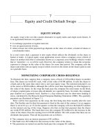
Figure 17.3 Capital gains/losses on a mandatorily exchangeable at maturity
the bond for shares at maturity, using an exchange ratio formula that can produce a lower rate
of participation in any rise in the share price compared to purchasing the actual shares in the
first instance. For example, a deal might be structured along the lines shown in Table 17.5.

The solid line in Figure 17.3 shows the capital gain or loss an investor would make on this
ME at maturity for a range of different possible share prices. The assumption is that the investor
has purchased a bond for $100 when it was issued. The dotted line shows the capital gains and
losses the investor would have achieved if he or she had used the $100 to buy one ABC share
in the first instance. A few examples will help to explain the ME bond values in the graph.
r
Share price at maturity = $75. The investor receives one share worth $75 and the capital
loss on the bond is $25.
r
Share price at maturity = $100. The investor receives one share worth $100 and there is no
capital gain or loss on the bond.
r
Share price at maturity is between $100 and $125. The investor receives shares to the value
of $100. The capital gain on the bond is zero.
r
Share price at maturity =$150. The investor receives 0.8 shares worth $120 and the capital
gain on the bond is $20. This is $30 less than the gain would have been if the investor had
purchased one ABC share for $100 in the first instance.
Convertible and Exchangeable Bonds 185
r
Share price at maturity =$200. The investor receives 0.8 shares worth $160 and the capital
gain is $60. This is $40 less than it would have been if the investor had purchased one ABC
share rather than the bond at the outset.
At share prices higher than $125 the investor in the ME bond begins to participate in further
increases in the share price, but to a lesser extent than if he or she had bought shares in the first
instance. Also the bond does not offer the kind of capital protection afforded by a traditional
convertible or exchangeable bond. However it does pay a high coupon rate of 5% p.a. while
the underlying share pays no dividends. The investor has the benefit of this income advantage
for three years and then the bond has to be exchanged for shares. In a flat share market with
little opportunities for capital growth this may be a major plus point. The coupon income also

provides some offset against a possible fall in the value of the shares over the three years.
CHAPTER SUMMARY
A convertible bond (CB) can be converted into a fixed number of shares of the issuer, at the
decision of the holder. The number of shares acquired is determined by the conversion ratio.
The parity value of a CB is its value considered as a package of shares, i.e. the conversion ratio
times the current share price. The bond floor is its value considered purely as a bond. A CB
should not trade below its bond floor or its parity value, assuming that immediate conversion
is possible. Its value over-and-above parity is called conversion premium.
Conversion premium is affected by the value of the call option that is embedded in a CB.
At a low share price it is unlikely that the bond will be converted and it trades close to its bond
floor. Conversion premium is high. At a high share price conversion is likely and the bond will
trade close to its parity value. Conversion premium is low.
CBs are bought by investors who wish to profit from increases in the share price but who do
not wish to suffer excessive losses if it falls. They are also bought by hedge funds as a means
of acquiring relatively inexpensive options. In practice, valuing a CB can be complex. It often
incorporates ‘call’ features that allow the issuer to retire the bond before maturity, sometimes
to force conversion. An exchangeable bond is issued by one organization and is exchangeable
for shares in another company. They are sometimes issued by an organization that has acquired
an equity stake in another business; rather than sell the shares outright it raises cheap debt by
selling bonds exchangeable for those shares. An investor who buys a mandatory convertible or
exchangeable bond is obliged to acquire shares at some future point in time. The bond may be
structured such that the investor receives a high coupon or has some level of capital protection.

18
Structured Securities: Examples
INTRODUCTION
One of the strengths of derivatives is that they can be combined in many ways to create new risk-
management solutions. Similarly, banks and securities houses can use derivatives to create new
families of investments aimed at the institutional and retail markets. Products can be developed
with a wide range of risk and return characteristics, designed to appeal to different categories

of investors in different market conditions. The choice is no longer limited to buying bonds,
investing in shares or placing money in a deposit account. Derivative instruments can create
securities whose returns depend on a wide range of variables, including currency exchange
rates, stock market indices, default rates on corporate debt, commodity prices – even electricity
prices or the occurrence of natural disasters such as earthquakes.
Some structured products are aimed at the more cautious or risk-averse investor. They
incorporate features that protect at least some percentage of the investor’s initial capital. Others
actually increase the level of risk that is taken, for those who wish to achieve potentially higher
returns. A classic (and infamous) example is the ‘reverse floater’ whose value moves inversely
with market interest rates. The problem is that it may also incorporate a significant amount of
leverage, so that if interest rates rise the potential losses are enormous. In 1994 Orange County
in California lost over $1.6 billion through such investments.
Derivatives also allow financial institutions and corporations to ‘package up’ and sell off
risky positions to investors who are prepared to take on those risks for a suitable return.
Chapter 17 gave an example of the technique. A company that owns a cross-holding in another
firm’s equity can issue an exchangeable bond. The company benefits from cheaper borrowing
costs and (assuming exchange takes place) will never have to pay back the principal value. The
bond could be structured as a mandatorily exchangeable, such that the shares are definitely
sold off on a future date at a fixed price but with the proceeds from the sale received up
front.
There are literally thousands of ways in which derivatives can be used to create structured
securities and only a few examples can be explored in an introductory text such as this. The
first sections in this chapter discuss a very typical structure, an equity-linked note with capital
protection. We look at a number of different ways in which the product can be constructed to
appeal to different investor groups, and at the actualcomponents that are used in its manufacture.
The final sections explore structured securities whose returns are linked to the level of default
on a portfolio of loans or bonds. This is one of the largest growth areas in the modern financial
markets.
CAPITAL PROTECTION EQUITY-LINKED NOTES
We begin with an equity-linked note (ELN) – a product that offers investors capital protection

plus some level of participation in the rise in the value of a portfolio or basket of shares. When
188 Derivatives Demystified
sold into the retail market the return on these products is usually linked to the level of a well-
known stock market index such as the S&P 500 or the FT-SE 100. An index like this simply
tracks the change in the value of a hypothetical portfolio of shares. The notes can also be given
a ‘theme’ selected to be attractive to investors at a particular moment in time. For example,
the payoff might depend on the value of an index of smaller company shares or of technology
stocks. The notes we will assemble in this chapter are based on a portfolio of shares currently
worth €50 million. The total issue size is €50 million, the notes mature in two years’ time
and their maturity value will be calculated as follows:
Maturity value of notes = (Principal invested × Capital protection level)
+ (Principal invested × Basket appreciation × Participation rate)
For example, suppose we issue the notes with 100% capital protection and 100% participation
in any increase in the value of the portfolio over two years. If at maturity the basket of shares is
worth €40 million, then the investors get back their €50 million and suffer no loss of capital.
But if the basket has risen in value by (say) 50%, then the investors are paid €75 million.
Maturity value = (€50 million × 100%) + (€50 million × 50% × 100%)
= €75 million
The first step in assembling the notes is to guarantee the investors’ capital. The strategy
here is to take some proportion of the €50 million raised by selling the notes and invest the
money for two years, so that, with interest, it will grow to a value of exactly €50 million at
maturity. Suppose we identify a suitable fixed-rate investment that pays 5.6% p.a. with interest
compounded annually. If, in that case, we deposit about €44.84 million the investment will
be worth €50 million at maturity in two years. This can be used to guarantee the €50 million
principal on the structured notes.
How can we also pay the investors a return based on any appreciation in the value of the
portfolio? Clearly we cannot buy the actual shares since most of the money collected from the
investors has been used to guarantee the capital repayment.
The answer is that we buy a European call option that pays off according to the value of
the basket of shares in two years’ time, the maturity of the structured notes. The strike is set

at-the-money at €50 million. Suppose the portfolio at maturity is worth €75 million, a rise of
50% from the starting value. Assuming 100% capital protection and 100% participation, we
would then have to pay the investors €75 million at maturity. However, we are covered. We
have €50 million from the maturing deposit and the intrinsic value of the call would be €75
million − €50 million = €25 million.
The next step is to contact our option dealer and purchase a two-year at-the-money European
call on the basket of shares. Suppose that the dealer quotes us a premium of €8.6 million for
the contract. Then it is clear that we cannot offer investors 100% capital protection and 100%
participation in any rise in the value of the portfolio. We collected €50 million from investors
and deposited €44.84 million, which leaves only €5.16 million. If the investors demand the
full capital guarantee, we will need to spend less money on the option contract. In fact the
premium we are able to pay determines the participation rate we can offer to the investors in
the notes. We know that €8.6 million buys 100% participation; therefore our budget will only
buy a maximum participation rate of 60%.
Maximum participation rate = €5.16 million / €8.6 million = 60%
Structured Securities: Examples 189
EXPIRY VALUE OF 100% CAPITAL PROTECTION NOTES
Table 18.1 shows the value of the equity-linked notes at maturity in two years’ time, on the
basis that they are offered with 100% capital protection and a 60% participation rate. The first
column shows a range of possible values the basket may take at maturity; the second shows
the percentage change starting from €50 million. The final three columns show the value of
the notes and the capital gain or loss investors in the notes have made at maturity.
Some examples from the table will help to explain the figures. Let us suppose that the basket
at maturity is worth €50 million or €60 million.
r
Basket Value €50 million. The notes offer 100% capital guarantee, so investors get back
their original €50 million. As the change in the value of the basket is zero, investors receive
no additional payment. Their capital gain/loss is zero.
r
Basket value €60 million. Investors are repaid their €50 million. The basket has risen in

value by 20%, the participation rate is 60% so they are also paid an additional €50 million
× 20% × 60% = €6 million. The capital gain for the investors is 60% × 20% = 12%.
The solid line in Figure 18.1 shows the percentage capital gains or losses on the notes
over the two years to maturity, for a range of different values of the basket at that point. The
dotted line shows the percentage rise in the basket. If the basket at maturity is worth (say) €80
million then an investor who had purchased the underlying shares in the first instance would
have achieved a capital gain of 60%.
Table 18.1 Maturity value of 100% capital protection equity-linked note
Basket value at Basket ELN maturity Capital Capital gain
maturity (€) change (%) value (€) gain/loss (€) loss (%)
40 000 000 −20 50 000 000 0 0
50 000 000 0 50 000 000 0 0
60 000 000 20 56 000 000 6 000 000 12
-60%
-40%
-20%
0%
20%
40%
60%
20 30 40 50 60 70 80
Basket value at maturity million
Capital gain/loss
ELN
Basket
Figure 18.1 Capital gain/loss on 100% capital guarantee note
190 Derivatives Demystified
An investor in the equity-linked notes would have made 60% of this, i.e. 36%. On the other
hand, if the basket is only worth €20 million at maturity then an investor in the shares would
have lost 60% of their capital while a purchaser of the notes would have lost none. Note that this

analysis only considers capital gains and losses; the notes do not pay any dividends or interest.
Potential investors could buy the underlying shares and earn dividend income, or deposit the
cash with a bank and earn interest.
100% PARTICIPATION NOTES
Some investors prefer to have a lower level of capital protection but a higher degree of par-
ticipation. Suppose that we decide to offer a 100% participation rate. We saw before that this
requires an expenditure of €8.6 million to purchase a call option. From this we can calculate
how much there remains from the €50 million to place on deposit, and the proceeds in two
years’ time at a return of 5.6% p.a. This calculation shows that we can only afford to guarantee
a repayment of €46.2 million at maturity, which is roughly 92% of the initial capital provided
by the investors.
Figure 18.2 shows capital gains and losses on 92% capital protection and 100% participation
notes for a range of possible basket values at maturity. If the shares are worth €50 million
investors are repaid 92% of their capital (a loss of 8%). If an investor had bought the actual
shares the capital loss would have been zero. On the other hand, the maximum loss on the
notes is 8% while 100% could potentially be lost on the shares.
If the basket is worth more than €50 million at maturity, the advantage of the higher
participation rate becomes apparent. For example, if it is worth €80 million these notes produce
a capital gain of 52%. This compares favourably with 36% on the 100% capital protection notes
(though unfavourably with a direct investment in the basket which would have returned a 60%
capital gain).
One possibility, of course, is to offer different classes of notes aimed at different purchasers,
some with higher capital protection aimed at the more risk-averse and 100% participation notes
-60%
-40%
-20%
0%
20%
40%
60%

20 30 40 50 60 70 80
Basket value at maturity million
Capital gain/loss
ELN
Basket
Figure 18.2 Capital/gain loss on 100% participation equity-linked note
Structured Securities: Examples 191
aimed that those who are prepared to take a little more risk for potentially higher rewards. Note
that the securities we have been structuring so far in this chapter function in essence rather like
exchangeable bonds. There is a level of capital protection plus an equity-linked return.
CAPPED PARTICIPATION NOTES
It is possible to offer investors 100% capital protection and at the same time 100% participation
in any rise the value of the basket of shares, at the cost of capping the profits on the notes. How
can we establish the level of the cap? The strategy involves selling an out-of-the money call
on the basket and receiving premium. This increases the amount of money available to buy the
at-the-money call on the basket. The other side of the coin is that the profits on the notes must
be capped at the strike of the call that is sold. We know how much money has to be raised from
selling such an option.
Cash raised from issuing notes = €50 million
Deposited for 100% capital protection = €44.84 million
Premium cost of long call for 100% participation = €8.6 million
Shortfall = €3.44 million
This tells us that we must write a call on the basket of shares with a strike set such that the
buyer is prepared to pay us a premium of €3.44 million. Suppose we contact an option dealer
and agree to write a call on the basket struck at a level of €67.5 million, which raises exactly
the required amount of money. The strike is 35% above the spot value of the basket.
The overall effect is that we can promise 100% capital protection and 100% participation
in any rise in the basket, but the capital gain on the notes must be limited to €17.5 million,
or a 35% return based on the initial capital of €50 million. We purchased a call on the basket
struck at €50 million. However, any gains on the shares beyond a value of €67.5 million will

have to be paid over to the buyer of the €67.5 million strike call.
Figure 18.3 compares the capital gains and losses on the capped equity-linked notes to what
investors would have achieved if they had invested the money in the actual shares. To see how
-20%
0%
20%
-40%
-60%
40%
60%
20 30 40 50 60 70 80
Basket value at maturity million
Capital gain/loss
ELN
Basket
Figure 18.3 Capital/gain loss at maturity on capped equity-linked note
192 Derivatives Demystified
this works out for investors, we can take some values from the graph. These are based on
different possible values of the basket at the maturity of the notes.
r
Basket value €40 million. As the notes offer a 100% capital guarantee, investors are repaid
€50 million. The capital loss is zero. On the other hand, if they had bought the actual shares
they would have lost €10 million or 20% of their capital.
r
Basket value €60 million. The investors are repaid their €50 million initial capital. The basket
has risen by 20% and the participation rate is 100%, so they are also paid an additional €10
million for the rise in basket. The capital gain for the investors is 20%, as it would have been
if they had purchased the actual shares.
r
Basket value €80 million. The investors are repaid their €50 million capital. The basket has

risen in value by 60%. However the capital gain on the notes is capped at 35%. The total
amount repaid to investors at maturity is €67.5 million.
The capital gain on the notes is capped here at 35%, but the potential gains if the actual shares
had been purchased by the investors is unlimited. On top of this, of course, the shares would
pay dividends which can be re-invested, whereas the notes pay no interest at all. They could
be structured to include interest payments, but some other feature would have to be adjusted.
For example, the capital protection level could be reduced, or the level of the cap lowered.
AVERAGE PRICE NOTES
One concern that investors might have about purchasing the equity-linked notes is that the
basket could perform well for most of the two years to maturity, and then suffer a serious
collapse towards the end. This sort of problem is illustrated in Figure 18.4. The portfolio is
worth €50 million at the outset and, with some ups and downs, is trading comfortably above
that level with only a few months to the expiry of the notes. However, it then suffers a slump.
In all of the versions of the equity-linked notes considered so far in this chapter, the investors
30
40
50
60
70
012
Time in years
million
Basket value
Figure 18.4 Potential price path for the basket over two years
Structured Securities: Examples 193
would not benefit from those interim price rises. The payout is based solely on the value of the
basket at maturity.
One way to tackle this problem is to use an average price or Asiatic call option when
assembling the notes. The value of a fixed strike average price call option at expiry is zero,
or the difference between the average price of the underlying and the strike, whichever is the

greater. These contracts are specifically designed to help with the sort of concerns investors
may have about the equity-linked notes, since the payout would not be based on the value of
the basket at a specific moment in time, the expiry date, but its average value over some defined
period of time. This could be the three- or the six-month period leading up to expiry, or even
the whole life of the option contract. The averaging process can be based on daily or weekly
or monthly price changes.
Average price options have another advantage of great practical importance to structurers
assembling products such as equity-linked notes. All other things being equal, an average
price option tends to be cheaper than a standard vanilla option. The reason, again, relates
to volatility. The averaging process has the effect of smoothing out volatility. To put it an-
other way, the average value of an asset over a period of time tends to be relatively stable,
more so than the cash price over the same period. (This assumes that the movements follow
a random path, so that price rises and falls tend to cancel out to some extent.) The more fre-
quently the averaging process is carried out, the better the smoothing effect. All other things
being equal, an average price option with daily averaging is cheaper than one with weekly
averaging.
We know that to structure the notes with 100% capital protection we must deposit €44.84
million. Using vanilla call options, we need €8.6 million to offer a 100% participation rate.
The reason for adjusting the notes in various ways – e.g. lowering the participation rate or
capping the profits – is that there is not enough cash available to do both. However, with the
same values used to price the vanilla option the cost of buying an average price option from
a dealer could actually come in within budget. We could offer a 100% capital guarantee plus
100% participation in any increase in the average value of the basket.
LOCKING IN INTERIM GAINS: CLIQUET OPTIONS
Average rate options are very useful but they are not likely to help if the shares first perform
well and then very badly indeed for a sustained period of time leading up to maturity. The
chances are that the average price would be below the strike. One solution to this problem,
although it is likely to be expensive, is to use a cliquet or ratchet option when assembling
the notes. A cliquet is a product that locks in interim gains at set time periods, which cannot
subsequently be lost. Suppose, this time, that when assembling the equity-linked notes we buy

a cliquet option, consisting of two components:
1. A one-year European call starting spot with a strike at the current spot value of the basket
€50 million. This is a standard call option.
2. A one-year European call, starting in one year, with the strike set at the spot value of the
basket at that point in time. This is known as a forward start option.
To help to explain the effect of the cliquet, Figure 18.5 shows one potential price path for the
basket of shares over the next two years. The value starts at €50 million. At the end of one
year it is worth approximately €55 million. The first option in the cliquet, the spot start call,
will expire at that point and will be worth €5 million in intrinsic value. This cannot be lost.
194 Derivatives Demystified
30
35
40
45
50
55
60
65
70
01 2
Time in years
million
Basket value
Basket value = 55 million
Gain locked in = 5 million
Figure 18.5 Possible price path for the basket and locked-in gain
Now the strike for the second option in the cliquet, the forward start option, will be set at €55
million. At the expiry of that option the basket in this example is worth less than €55 million,
so it expires worthless. If the basket at expiry was worth more than €55 million then gains
would be achieved in addition to the €5 million locked in.

The problem with the cliquet is of course the cost of the premium. It actually consists of
two call options each with one year to maturity, one starting spot and the other starting in one
year’s time. This is more expensive than a standard two-year call option because it provides
additional flexibility. The result is that if the cliquet is used, the capital protection level on the
notes would have to be lowered, or the participation rate cut, or the returns capped.
SECURITIZATION
In these final examples we look at structured bonds whose returns are linked to the level of
default on a pool of assets. Generally, securitization is the process of packaging up assets such
as mortgages and bank loans and selling them off to capital markets investors in the form
of bond issues. The bondholders are paid out of the cash flow stream from the underlying
assets. The growth in securitization has been one of the most significant developments in
finance over the past decade. Issuance in the European market in 2002 totalled €157.7 billion,
according to the European Securitization Forum – a body formed of major participants in the
business.
Investment bankers have become increasingly creative about the types of assets that are given
the securitization treatment. It seems that almost anything that generates future cash flows that
can be forecast with a reasonable degree of accuracy can be packaged up and sold into the
public bond markets. Bonds have been issued that are backed by the royalty and copyright
payments due to rock stars (so-called Bowie bonds). Italy has issued bonds backed by future
ticket sales at art galleries and by future collections of unpaid tax. Soccer clubs have borrowed
against receipts due from season ticket sales. Even whole companies have been securitized,
notably in the UK chains of managed pubs.
Structured Securities: Examples 195
The basic process of securitization usually tends to fall into a fairly standard pattern. Firstly,
a set of assets is identified that will generate a stream of future cash flows. Secondly, the assets
are sold by their owner to an entity known as a special purpose vehicle (SPV). The purpose of
the SPV is to issue bonds, and with the proceeds purchase the assets from the original owner.
The cash flow stream from the assets is used to service the interest and principal payments due
on the bonds.
The bonds are usually rated by one or more of the major ratings agencies. If the underlying

assets are of poor quality and there is risk that the cash flow stream may not be sufficient to
pay back the bondholders, then it is necessary to use what are known as credit-enhancement
techniques to make the bonds more attractive. A common method is to issue different classes
or tranches of bonds with different risk-return characteristics.
For example, there may a tranche with the highest credit rating AAA, which means that
investors have a very high probability of being paid. Further tranches will have lower credit
ratings but will pay high coupons in compensation. If the assets do not generate sufficient cash
flows then the lowest-rated bonds suffer first. Often at the bottom of the pile there is a so-called
equity investor who earns a return if there is anything left after all the other classes of investors
have been paid.
Figure 18.6 shows a typical securitization structure. The underlying assets are bank loans
originated by a commercial bank. The bank would like to sell off the assets, partly because
it wishes to free up capital to create further loans; and partly because it wishes to reduce
the level of credit or default risk it retains on its balance sheet. A bank that holds loans
that carry the risk of default has to set aside capital to cover this eventuality. This can ad-
versely affect important performance ratios such as return on equity. So the bank sells the
loan portfolio to a company (the SPV) specifically set up for the purchase, with the help of
its investment banking advisers and lawyers. The SPV raises the cash to buy the loans from
the bond investors, who are repaid via the SPV from the cash flows from the underlying
loans.
Why would investors buy the bonds? Because the issue is set up in such a way that they
receive a return they believe is attractive in relation to the risks being taken. Since the underlying
assets in this example are bank loans, the main risk to the investors is that of a significant level
BOND
INVESTORS
BANK
(ORIGINATOR)
SPV
LOANS
(ASSETS)

Payment for purchase of assets
Cash flows
from assets
Coupons + Principal
Proceeds from selling bonds
Figure 18.6 Securitization of bank loans
196 Derivatives Demystified
of default. This could mean that the SPV is unable to pay some coupons on the bonds, or even
that the bondholders’ capital is at risk.
The system of creating different tranches of bonds with different risk and return character-
istics helps in such circumstances. The more risk-averse investors can buy the highest-rated
tranche, making their investment very secure. Others may be prepared to buy the lower-rated
tranches which pay higher coupons but suffer first if the underlying loans default. Another
method often used in securitization is known as over-collateralization. In effect the loan assets
transferred to the SPV are increased so that a certain level of default in the loan portfolio is
allowed for.
The main advantage of using an SPV from the perspective of investors is that the assets are
segregated and transferred from the ownership of the originator of those assets – in the example,
from the commercial bank. The bond investors are only exposed to the credit or default risk on
the assets, which may be easier to assess and monitor. If they purchased bonds issued directly by
the commercial bank rather than by the SPV they would be exposed to a much wider set of risks –
for example, the risk that the bank as a whole is mismanaged and is unable to repay its debt.
SYNTHETIC SECURITIZATION
There are occasions, however, when a bank does not wish to sell a loan portfolio outright. It
may consist of commercial loans to important corporate clients, and for relationship reasons it
would be difficult to transfer the ownership to another party. There may be other tax, legal and
regulatory constraints. However, if the bank retains the ownership of the loans on its balance
sheet it is exposed to the risk of default and has to set capital aside against this risk. Derivative
products can provide a range of alternative solutions; this time we will use a credit default
swap (CDS). As we saw in Chapter 7, a CDS has two parties: the protection seller and the

protection buyer.
r
Protection buyer. The protection buyer pays a premium of so many basis points per annum
to buy protection on a referenced bond or loan or portfolio of loans.
r
Protection seller. If a defined credit event occurs during the life of the contract, the protection
buyer either receives a cash compensation payment or delivers the asset to the protection
seller in return for a defined payment.
r
Credit event. A credit event is anything defined in the CDS contract that triggers the com-
pensation payment or the delivery of the asset to the protection seller. Typical events include
non-payment on due obligations and ratings downgrades.
Figure 18.7 illustrates a synthetic securitization deal involving a commercial bank. This
time the bank does not physically sell the assets to an SPV, but instead buys protection from
the SPV on the assets or some proportion of the assets using a credit default swap. It pays an
annual premium to the SPV for the protection. The SPV issues bonds to investors and uses the
proceeds to buy Treasury securities.
The investors in the bonds issued by the SPV earn a return in addition to the return on the
Treasuries because of the premium paid to the SPV by the bank. The bank pays the premium
for the protection it receives as the buyer of protection under the CDS contract. As the seller
of protection, the SPV will have to make compensation payments to the bank if credit events
are triggered, i.e. defaults on the portfolio of loans. Since it has no other assets it would have
to sell some of its stock of Treasury bonds to achieve this, thus reducing the cash available to
pay back the investors.
Structured Securities: Examples 197
BOND
INVESTORS
BANK
(ORIGINATOR)
SPV

LOANS
(ASSETS)
Premium
Cash
flows
from
assets
Coupons + Principal
Cash from sale of bonds
Payment if credit
event triggered
TREASURIES
Treasury return
CDS
Figure 18.7 Synthetic securitization
This structure is called a synthetic securitization because the bank does not physically sell
the assets. Instead it retains them on its balance sheet but purchases protection against default
by entering into the credit default swap with the SPV. Normally some elements of credit
enhancement will be incorporated into the structure to encourage investors to buy the bonds.
The commercial bank may agree to suffer the first losses on the loan portfolio up to a certain
level before any payment from the SPV is triggered under the terms of the CDS. In addition,
the bonds issued by the SPV will normally be structured into different tranches, such that the
lower-rated bonds will suffer before the higher-rated bonds are affected.
CHAPTER SUMMARY
Derivatives are not only used in risk management and in trading applications. They are also
used to create a very wide range of so-called structured securities whose returns to investors
depend on such factors as the value of a basket of shares, currency exchange rates or the level
of interest rates over some period of time. Banks can also use derivatives to package up the
risks they acquire as part of their business operations and ‘sell them off’ to investors who are
prepared to assume the risks for a suitable return.

The equity-linked note, which goes by a variety of brand names, is a typical structured
product and is now offered to retail investors as well as to institutions. Normally the investors
are offered a level of capital protection plus participation in any rise in the value of an equity
index or a specific basket of shares. The product can be assembled by depositing a sum of
money to guarantee the principal repayment and buying a call on the index or basket. The gain
on the note may be capped or based on the average value of the index or basket, or it may be
structured such that interim gains are locked in.
Securitization is the process of assembling assets such as loans and selling bonds to investors
that are repaid from the cash flows generated by the assets. Usually the assets are transferred
into a special purpose vehicle which exists simply to collect cash and pay interest and principal
to the bondholders. Typically, different tranches or ‘slices’ of bonds are sold with different
198 Derivatives Demystified
risk-return characteristics and different credit ratings. Sometimes the assets used are existing
bonds which are trading cheaply in the market because they are unpopular in some way.
Securitization deals have also been based on the cash flows due from future trade receivables,
ticket sales, taxation, royalty and copyright payments and the revenues from managed pub
chains.
A bank that does not wish to sell a loan book physically can enter into a synthetic securiti-
zation deal. Here it buys protection against default on some proportion of its loan book from
an SPV and pays a fee or premium. The SPV uses this premium to pay its bond investors a
return above and beyond that on Treasury bonds. The downside is that investors will suffer
losses if there is a significant level of default on the bank’s loan book.
Appendix A
Financial Calculations
TIME VALUE OF MONEY
Time value of money (TVM) is a key concept in modern finance. It tells us two things:
r
A dollar received today is worth more than a dollar to be received in the future.
r
A dollar to be received in the future is worth less than a dollar received today.

The reason for this is because a dollar today can be invested at a rate of interest and will grow
to a larger sum of money in the future. The cost of money for a specific period of time (its time
value) is measured by the interest rate for the period. Interest rates in the financial markets are
normally quoted on a nominal per annum basis. A nominal interest rate has two components:
r
Real rate. This compensates the lender for the use of the funds over the period.
r
Inflation rate. This compensates the lender for the predicted erosion in the value of money
over the period.
Normally the inflation element is more subject to change than the real or underlying rate.
The relationship between the two can be expressed mathematically (with the rates inserted in
the formulae as decimals):
1+ Nominal rate = (1+ Inflation rate) × (1 + Real rate)
Real rate = [(1+ Nominal rate)/(1 + Inflation rate)] − 1
If the nominal interest rate for one year is 5% p.a. (0.05 as a decimal) and the predicted rate of
inflation over the period is 3% p.a. (0.03 as a decimal) then the real interest rate is calculated
as:
Real rate = (1.05/1.03) − 1 = 0.0194 = 1.94% p.a.
By convention, interest rates are usually expressed per annum, even if the borrowing or lending
period is shorter than a year. To calculate the interest due on a loan or deposit that matures in
less than one year the annualized rate must be reduced in proportion.
FUTURE VALUE (FV)
Suppose we deposit $100 for one year with a bank. The interest rate paid is 10% p.a. simple
interest, that is, without compounding. The principal amount invested is called the present
value (PV). The principal plus interest at the maturity of the deposit is called the future value
(FV). The interest rate expressed as a decimal (10 divided by 100) is 0.1.
Future value (FV) = Principal + Interest at maturity
= 100 + (100 × 0.1) = 100 × 1.1 = 110
Interest at maturity = 100 × 0.1 = 10
200 Derivatives Demystified

This is a simple interest calculation because there is no compounding or ‘interest on interest’
involved in the formula. Note that if we deposit $100 for one year and our account is credited
with $110 at maturity, we could work out that the simple interest return earned on the investment
is 10% p.a. Suppose now we invest $100, but this time for two years at 10% p.a. and interest
is compounded at the end of each year. What is the future value (FV) after two years? At the
end of one year there is 100 ×1.1 = $110 in the account. Therefore, to work out the FV at the
end of two years we multiply this by 1.1 again.
Future value (FV) = Principal + Interest
= 100 × 1.1 × 1.1 = 100 × 1.1
2
= 121
Because of compounding we now have $21 in interest. The first year’s interest was $10. The
second year’s interest is $11. In addition to interest on the original principal of $100, we have
earned $1 interest on interest. The general formula for calculating present value when interest
is compounded periodically is:
FV = PV × (1 + r/m)
n
where FV = future value
PV = present value
r = the interest rate p.a. as a decimal (the percentage rate divided by 100)
m = the number of times interest is compounded per year
n = the number of compounding periods to maturity = years to maturity × m
In the previous example interest was compounded only once a year and it is a two-year
deposit, so the values are:
r = 0.1
r/m = 0.1/1 = 0.1
n = 2
PV = 100
FV = 100 × 1.1
2

= 121
There are many types of investment where interest is compounded more than once a year. For
example, the calculations for US Treasury bonds and UK gilts are based on six-monthly periods,
known as semi-annual compounding. Other investments pay interest every three months. Credit
cards often charge interest on unpaid balances on a monthly basis. Suppose we invest $100
for two years at 10% p.a. Interest is compounded every six months. What is the future value
at maturity in this case?
FV = 100 × (1 + 0.1/2)
4
= 121.55
The annual rate expressed as a decimal is divided by two to obtain a six-monthly rate. Com-
pounding is for four half-yearly periods. The future value is higher than when interest was
compounded annually. This illustrates a basic principle of TVM. It is better to earn interest
sooner rather than later, since it can be re-invested and will grow at a faster rate.
ANNUAL EQUIVALENT RATE (AER)
Because interest rates in the market are expressed with different compounding frequencies it
is important to be very careful when comparing rates. For example, suppose we are offered
Appendix A 201
Table A.1 Nominal rate 10% p.a.
Compounding frequency Annual equivalent rate
(% p.a.)
Annually 10.0000
Semi-annually 10.2500
Quarterly 10.3813
Monthly 10.4713
Weekly 10.5065
Daily (365 times per annum) 10.5156
two investments. The maturity in both cases is one year, but the first investment offers a return
of 10% p.a. with interest compounded annually. The second offers a return of 10% p.a. with
interest compounded semi-annually. Which should we choose?

The answer is the semi-annual investment, since the interest paid half-way through the year
can be re-invested for the second half of the year. And yet the quoted or nominal interest
rate (10% p.a.) looks exactly the same in both cases. This tells us that a nominal 10% p.a.
interest rate with semi-annual compounding cannot be directly compared with a 10% p.a.
rate with annual compounding. In fact 10% p.a. with semi-annual compounding is equivalent
to 10.25% p.a. with annual compounding. This can be demonstrated using the future value
formula. Suppose we invest $1 for a year at 10% p.a. with semi-annual compounding. The
present value is $1. The future value at maturity is calculated as:
FV = $1 × (1 + 0.1/2)
2
= $1.1025
Interest at maturity = $1.1025 − $1 = $0.1025
This is same amount of interest we would receive if we invested $1 for one year at 10.25%
p.a. with annual compounding. This calculation is the basis for what is known as the annual
equivalent rate (AER) or the effective annual rate. A rate of 10% p.a. with semi-annual com-
pounding is equivalent to 10.25% p.a. with annual compounding. Table A.1 sets out some other
examples. For example, a nominal or quoted interest rate of 10% p.a. with daily compounding
is equivalent to 10.5156% p.a. with interest compounded once a year.
The following formula will convert between nominal and annual equivalent rates:
r
ann
= (1 +r
nom
/m)
m
− 1
where r
ann
= the annual equivalent rate p.a. as a decimal
r

nom
= the nominal interest rate p.a. as a decimal
m = the number of times interest is compounded a year.
Once potential source of confusion in the financial markets is the way that people refer to
interest rates. A rate said to be ‘10% semi-annual’ does not usually mean an interest rate of
10% every six months. It normally means a rate of 10% p.a. with semi-annual compounding.
The rate every six months is actually half of 10% which is 5%.
As interest is compounded more and more frequently the annual equivalent rate approaches
a limit. This is defined by what is known as continuous compounding, a method of calculating
interest widely used in the derivatives markets. The effective annual equivalent rate where
interest is compounded continuously can be calculated as follows (all rates are expressed as
202 Derivatives Demystified
decimals in the formula):
r
ann
= e
rcont
− 1
where r
ann
= the annual equivalent rate (AER) p.a.
r
cont
= the nominal rate of interest p.a. with continuous compounding
e = the base of natural logarithms
∼
=
2.71828.
A nominal 10% p.a. rate with continuous compounding is equivalent to approximately
10.5171% p.a. with annual compounding. The EXP() function in Excel calculates e to the

power of the value in the brackets.
PRESENT VALUE (PV)
So far we have looked at calculating a future value given a present value and a rate of interest.
It is also possible to calculate the value in today’s terms of a cash flow due to be received in
the future. The basic time value of money formula with periodic compounding is:
FV = PV × (1 + r/m)
n
Rearranging:
PV = FV/(1 +r/m)
n
In this version of the formula r is known as the discount rate. This formula allows us to calculate
the value in today’s terms of cash to be received in the future. This has very wide applications
in financial markets. For example, a debt security such as a bond is simply a title to receive
future payments of interest and principal. The ‘coupon’ is the regular interest amount paid on
a standard or ‘straight’ bond issued by a government or a corporate. A zero-coupon bond pays
no interest at all during its life and trades at a discount to its par or redemption value.
Suppose you are deciding how much to pay for a 20-year zero-coupon bond with a par
value of $100. The return on similar investments is currently 10% p.a. expressed with annual
compounding. Applying the TVM formula, the fair value of the bond is calculated as:
PV = 100/1.1
20
= $14.8644
The discount rate is the return currently available on similar investments with the same credit
(default) risk and the same maturity. This establishes a required rate of return and hence a fair
value for the bond. Economists would call it the ‘opportunity cost of capital’ – the return that
would be achieved on comparable investments if money is not tied up in the bond.
This methodology is extended to pricing coupon bonds, i.e. bonds that make regular interest
payments during their life. Let us suppose that you buy a bond that pays an annual coupon
of 10% p.a. The par or face value is $100 and the bond has exactly three years remaining
to maturity. How much is it worth today, if the rate of return on similar investments in the

market is currently 12% p.a. expressed with annual compounding? The traditional valuation
methodology is to establish the cash flows on the bond, discount each cash flow at a constant
rate, then sum the present values.
r
The cash flow in one year is $10, an interest payment of 10% of the $100 face value. Its PV
discounted at 12% for one year is 10/1.12 = $8.9286.
r
The cash flow in two years is another interest payment of $10. Its PV discounted at 12% for
two years is 10/1.12
2
= $7.9719.
Appendix A 203
r
The cash flow in three years is a final $10 interest payment plus the payment of the bond’s
$100 face value, a total of $110. Its PV discounted at 12% for three years is 110/1.12
3
=
$78.2958.
The sum of the PVs is $95.2, which establishes a fair market price for the bond. The bond is
trading below its face value of $100 because it pays a fixed coupon of only 10% p.a. in a current
market environment in which the going annual return for investments of this kind is 12% p.a.
In economic terms, investors will tend to sell the bond and switch into the higher-yielding
investments now available, until its price is pushed below its $100 face value and stabilizes at
around $95.2.
Option pricing models tend to use continuously compounded rates to calculate future values
and also to discount future cash flows, such as the exercise or strike price of a European-style
call or put. Future and present values with continuously compounded rates are calculated as
follows:
FV = PV × e
rt

PV = FV × e
−rt
where FV = future value
PV = present value
r = the continuously compounded interest rate p.a.
t = time in years
e = the base of natural logarithms
∼
=
2.71828.
For example, the future value of $100 invested for one year at a continuously compounded
rate of 10% p.a. is calculated as follows:
FV = $100 × e
rt
= $100 × e
0.1×1
= $110.5171
The present value of $100 to be received in one year if the continuously compounded rate of
interest for the period is 10% p.a. is calculated as follows:
PV = $100 × e
−rt
= $100 × e
−0.1×1
= $90.4837
YIELD OR RETURN ON INVESTMENT
The basic time value of money formula with periodic compounding is as follows:
FV = PV × (1 + r/m)
n
Given a present value and a future value, it is also possible by rearranging the formula to
calculate the periodic rate of return achieved on an investment:

Rate of return p.a. = [
n
√
(FV/PV) − 1] × m
where FV = future value
PV = present value
m = the number of times that interest is compounded a year
n = the number of compounding periods to maturity = years × m.
Suppose we invest a present value of $100 for three years. The future value to be received at
maturity is $125. There are no intervening cash flows. The annualized rate of return expressed
204 Derivatives Demystified
with different compounding frequencies is calculated as follows:
Rate of return with annual compounding = [
3
√
(125/100) − 1] × 1
= 7.72% p.a.
Rate of return with semi-annual compounding = [
6
√
(125/100) − 1] × 2
= 7.58% p.a.
The rate of 7.58% p.a. is a semi-annually compounded rate. Its annual equivalent rate, i.e. its
equivalent expressed with annual compounding, is 7.72% p.a. A continuously compounded
rate of return can also be calculated from a present and a future value. Where r is a continuously
compounded rate, we have the following equation:
FV = PV × e
rt
The continuously compounded return can be calculated as follows:
Rate of return p.a. with continuous compounding = ln (FV/PV) ×(1/t)

where ln () = the natural logarithm of the number in brackets
t = time to maturity in years.
To take the previous example, suppose we invest $100 for three years and are due to receive
$125 at maturity. There are no intervening cash flows.
Rate of return with continuous compounding = ln (125/100) ×(1/3)
= 7.44% p.a.
A rate of 7.44% p.a. with continuous compounding is equivalent to 7.72% p.a. with annual
compounding. The Excel function used to calculate the natural logarithm of a number is LN().
It is the inverse of the EXP() function.
TERM STRUCTURE OF INTEREST RATES
In developed markets the minimum rate of return on an investment for a given maturity period
is established by the return on Treasury (government) securities. It is sometimes called the risk-
free rate because there is no risk of default. The term structure shows the returns on Treasury
zero-coupon securities for a range of different maturity periods. Why not use coupon-paying
securities? The problem is that the return on a coupon bond depends to an extent on the rate
at which coupons can be re-invested during the life of the security. To calculate a return it is
necessary to make assumptions about future re-investment rates. A zero-coupon bill or bond is
much simpler. Because there are no coupons, no assumptions need be made about re-investment
rates.
Zero-coupon rates are also known as spot rates, and working with spot rates has many
advantages. Firstly, as stated previously, they can be used to calculate future values without
making any assumptions about future re-investment rates. Secondly, they can be used as a
reliable and consistent means of discounting future cash flows back to a present value. A
one-year risk-free cash flow should be discounted at the one-year Treasury spot rate; two-year
risk-free cash flows should be discounted at the two-year Treasury spot rate; and so on. A
non-Treasury security such as a corporate bond is valued by discounting the cash flows at the
appropriate Treasury spot rates plus a premium or spread that reflects the credit and liquidity
risk of the bond. For example, if the bond pays a coupon in one year this should be discounted
Appendix A 205
at the one-year Treasury spot rate plus a spread; if it pays a coupon in two years this should be

discounted at the two-year Treasury spot rate plus a spread; and so on.
Just as importantly, spot rates can be used to calculate forward interest rates, which are used
in the pricing of interest rate forwards, futures, swaps and options. In the next section we show
how forward rates can be extracted from spot or zero-coupon rates.
CALCULATING FORWARD INTEREST RATES
Table A.2 shows spot or zero-coupon rates for different maturity periods, expressed with
annual compounding. These are based on interbank lending rates rather than Treasuries, so
they incorporate a spread over the risk-free Treasury spot rates. The first rate Z
0×1
is the rate
of return applying to a time period starting now and ending in one year. In our examples, cash
flows that occur in one year will be discounted at this rate. The second rate Z
0×2
is the rate of
return that applies to a time period starting now and ending in two years. Cash flows that occur
in two years will be discounted at that rate. The rate Z
0×3
is the three-year spot or zero-coupon
rate, the rate at which three-year cash flows will be discounted.
The forward interest rate between years one and two can be calculated from these values
using an arbitrage argument. We will call that forward rate F
1×2
. It is the rate of return that
applies to investments made in one year that mature two years from now. Also, if we were
discounting a cash flow that occurs in two years back to a present value one year from now,
then it should be discounted at F
1×2
. If we wished to discount this value back to a present value
now, it should be discounted at the one-year spot rate Z
0×1

.
Suppose we borrow $1 now for two years at the two-year spot rate of 5% p.a. We take this
cash and deposit the money for one year at 4% p.a., the one-year spot rate. Suppose further
that we could agree a deal with someone that allowed us to re-invest the proceeds from this
deposit in a year for a further year at (say) 8% p.a. with annual compounding. Our cash flows
in two years’ time would look like this.
r
Principal plus interest repaid on loan = $1 × 1.05
2
= $1.1025
r
Proceeds from one-year deposit at 4% p.a. re-invested for a further year at 8% p.a. = $1 ×
1.04 × 1.08 = $1.1232
This is an arbitrage. In two years’ time we repay $1.1025 on the loan but achieve $1.1232 by
investing the funds for a year and then rolling over the deposit for a further year. Since it is
unlikely that such ‘free lunches’ will persist for long, this tells us that it is unlikely that anyone
would enter into a deal that allowed us to re-invest for the second year at 8% p.a. The fair
forward rate F
1×2
is the rate for re-investing money in one year for a further year such that no
Table A.2 Spot or zero-coupon
rates expressed with annual
compounding
Spot rate Value (% p.a.)
Z
0×1
4.00
Z
0×2
5.00

Z
0×3
6.00
206 Derivatives Demystified
such arbitrage opportunity is available. For no arbitrage to occur the following equation must
hold:
(1 + Z
0×2
)
2
= (1 + Z
0×1
) × (1 + F
1×2
)
This equation says that the future value of the two-year loan at maturity at the two-year spot
rate must equal the proceeds from investing that money for one year at the one-year spot rate
re-invested for a further year at the forward rate that applies between years one and two. In our
example the values are as follows:
1.05
2
= 1.04 × (1 + F
1×2
)
therefore:
F
1×2
= 6.01% p.a.
A similar argument can be used to calculate F
2×3

, the forward rate of interest that applies
between years two and three. Suppose we borrow $1 for three years now at Z
0×3
.Weinvest
the $1 for two years at Z
0×2
. For no arbitrage to be available the forward rate between years
two and three must be such that the following equation is satisfied:
(1 + Z
0×3
)
3
= (1 + Z
0×2
)
2
× (1 + F
2×3
)
1.06
3
= 1.05
2
× (1 + F
2×3
)
therefore:
F
2×3
= 8.03% p.a.

Notice here that the forward rates are increasing with time. This is the typical situation
where the term structure of interest rates shows the spot rates increasing with time to maturity.
The market is building in expectations of rising interest rates in the future.
FORWARD RATES AND FRAs
Forward interest rates have to relate to the market prices of interest rate futures and forward rate
agreements, otherwise arbitrage opportunities may be available. This is because interest rate
futures and FRAs can be used to lock into borrowing or lending rates for future time periods.
For example, suppose we could arrange the following deals (the example ignores the effects of
bid/offer spreads and brokerage):
r
Borrow $100 000 for two years at the two-year spot rate 5% p.a.
r
Deposit $100 000 for one year at the one-year spot rate 4% p.a.
r
Sell a 1 × 2 year FRA on a notional $104 000 at a forward rate of 8% p.a.
The principal plus interest on the deposit in one year is $104 000. The effect of selling the
FRA on this amount is to lock in a re-investment rate of 8% p.a. for a second year. Table A.3
shows the proceeds from this strategy at maturity in two years, taking a range of possible
re-investment rates up to 12% p.a.
r
Column (1) is the principal plus interest on the initial $100 000 loan at maturity in two years
at a rate of 5% p.a. annually compounded.
r
Column (2) is the proceeds from depositing that money for one year at 4% p.a.
r
Column (3) has a number of possible levels the one-year rate could take in one year for
re-investing the proceeds of the deposit.
Appendix A 207
Table A.3 Arbitrage constructed if FRA rate is not set at the forward interest rate
(1) (2) (3) (4) (5) (6)

Loan repayment Deposit proceeds Re-investment Deposit proceeds FRA payment Net cash
end-year 2 end-year 1 rate end-year 2 end-year 2 end-year 2
($) ($) (% p.a.) ($) ($) ($)
−110 250 104 000 4 108 160 4160 2070
−110 250 104 000 6 110 240 2080 2070
−110 250 104 000 8 112 320 0 2070
−110 250 104 000 10 114 400 −2080 2070
−110 250 104 000 12 116 480 −4160 2070
Table A.4 No arbitrage if FRA is transacted at the forward interest rate
(1) (2) (3) (4) (5) (6)
Loan repayment Deposit proceeds Re-investment Deposit proceeds FRA payment Net cash
end-year 2 end-year 1 rate end-year 2 end-year 2 end-year 2
($) ($) (% p.a.) ($) ($) ($)
−110 250 104 000 4 108 160 2090 0
−110 250 104 000 6 110 240 10 0
−110 250 104 000 8 112 320 −2070 0
−110 250 104 000 10 114 400 −4150 0
−110 250 104 000 12 116 480 −6230 0
r
Column (4) calculates the proceeds of the deposit re-invested for a further year at the rate in
column (3).
r
Column (5) is the payment on the FRA, either positive or negative. For example, suppose
the one-year rate in one year is 4%. The FRA rate is assumed to be 8% and the notional
$104 000. We will receive a compensation payment on the FRA of 8% − 4% = 4% applied
to the notional of the FRA, which comes to $4160.
r
Column (6) is the sum of columns (1), (4) and (5).
The values in column (6) are always positive, whatever happens to interest rates in the future,
which shows that there is an arbitrage. It should not be possible for us to sell the 1 × 2 year

FRA at 8% p.a. The fair rate for selling the FRA is the forward rate F
1×2
which we calculated
in the previous section as 6.01% p.a. Table A.4 assumes that the FRA is sold at 6.01% p.a.,
and the arbitrage profit disappears.
FORWARD RATES AND INTEREST RATE SWAPS
An interest rate swap (IRS) is an agreement between two parties to exchange cash flows on
regular dates, in which the cash flows are calculated on a different basis. In a standard interest
rate swap, one payment leg is based on a fixed rate of interest and the other is based on a
floating or variable interest rate linked to a benchmark such as the London Interbank Offered
Rate (LIBOR). The floating rate is reset at regular intervals, such as every six months. The
notional principal used to calculate the payments is fixed.
It will be helpful in the following discussion to use discount factors. A discount factor is
simply the present value of $1 at the zero-coupon or spot rate to the receipt of that cash flow.
208 Derivatives Demystified
Table A.5 Spot rates and discount factors
Spot rate Value (% p.a.) Discount factor Value
Z
0×1
4.00 DF
0×1
0.96153846
Z
0×2
5.00 DF
0×2
0.90702948
Z
0×3
6.00 DF

0×3
0.83961928
Table A.6 Swap floating rate cash flows
Notional Value Floating cash flow
Year ($m) Rate (% p.a.) ($m)
1 100 Z
0×1
4.00 4.00
2 100 F
1×2
6.01 6.01
3 100 F
2×3
8.03 8.03
Table A.5 shows the discount factors based on the spot rates used in previous sections of this
appendix. The one-year spot rate is 4% p.a. The one-year discount factor at this rate is:
1/1.04 = 0.96153846
The two-year spot rate is 5% p.a. So the two-year discount factor at this rate is:
1/1.05
2
= 0.90702948
One advantage of using discount factors is that the present value of a future cash flow can
immediately be established by multiplying that cash flow by the discount factor for that time
period.
We will now explore the relationship between swap rates, discount factors and forward
rates. Let us assume that we are considering entering into an interest rate swap deal with the
following terms:
Notional principal: $100 million
Maturity: 3 Years
We pay: Fixed rate, annually in arrears

We receive: Floating rate, annually in arrears
Interest calculations: annually compounded rates
First floating rate setting: 4% p.a.
Under the terms of the swap, we would pay a fixed rate of interest on a notional principal
of $100 million annually in arrears for three years. Our counterparty would pay in return a
variable rate of interest on $100 million annually in arrears for three years. The question is:
What fixed rate of interest should we pay to make this a fair deal?
One answer to this question is to start by calculating the floating rate cash flows on the swap
(see Table A.6). Since we are receiving the floating rate, these are positive cash flows. The first
cash flow due at the end of Year 1 is based on the one-year spot rate of 4% p.a. The second cash
flow will be based on the one-year rate in one year’s time, which we assume is established by
the forward rate F
1×2
. The third and final cash flow will be based on the one-year rate in two