essentials of investments with s p bind in card phần 3 docx
Bạn đang xem bản rút gọn của tài liệu. Xem và tải ngay bản đầy đủ của tài liệu tại đây (1.09 MB, 77 trang )
Bodie−Kane−Marcus:
Essentials of Investments,
Fifth Edition
II. Portfolio Theory 5. Risk and Return: Past
and Prologue
© The McGraw−Hill
Companies, 2003
the slope of the CML based on the subperiod data. Indeed, the differences across subperiods
are quite striking.
The most plausible explanation for the variation in subperiod returns is based on the
observation that the standard deviation of returns is quite large in all subperiods. If we take
the 76-year standard deviation of 20.3% as representative and assume that returns in one year
are nearly uncorrelated with those in other years (the evidence suggests that any correlation
across years is small), then the standard deviation of our estimate of the mean return in any of
our 19-year subperiods will be 20.3/ , which is fairly large. This means that in
approximately one out of three cases, a 19-year average will deviate by 4.7% or more from the
true mean. Applying this insight to the data in Table 5.5 tells us that we cannot reject with any
confidence the possibility that the true mean is similar in all subperiods! In other words, the
“noise” in the data is so large that we simply cannot make reliable inferences from average re-
turns in any subperiod. The variation in returns across subperiods may simply reflect statisti-
cal variation, and we have to reconcile ourselves to the fact that the market return and the
reward-to-variability ratio for passive (as well as active!) strategies is simply very hard to
predict.
The instability of average excess return on stocks over the 19-year subperiods in Table 5.5
also calls into question the precision of the 76-year average excess return (8.64%) as an esti-
mate of the risk premium on stocks looking into the future. In fact, there has been consider-
able recent debate among financial economists about the “true” equity risk premium, with an
emerging consensus that the historical average is an unrealistically high estimate of the future
risk premium. This argument is based on several factors: the use of longer time periods in
͙ළළ19 ϭ 4.7%
157
Triumph of the Optimists
As a whole, the last 7 decades have been very kind
to U.S. equity investors. Stock investments have out-
performed investments in safe Treasury bills by more
than 8% per year. The real rate of return averaged
more than 9%, implying an expected doubling of
the real value of the investment portfolio about every
8 years!
Is this experience representative? A new book by
three professors at the London Business School, Elroy
Dimson, Paul Marsh, and Mike Staunton, extends the
U.S. evidence to other countries and to longer time
periods. Their conclusion is given in the book’s title,
Triumph of the Optimists*: in every country in their
study (which included markets in North America, Eu-
rope, Asia, and Africa), the investment optimists—those
who bet on the economy by investing in stocks rather
than bonds or bills—were vindicated. Over the long
haul, stocks beat bonds everywhere.
On the other hand, the equity risk premium is prob-
ably not as large as the post-1926 evidence from
Table 5.1 would seem to indicate. First, results from the
first 25 years of the last century (which included the
first World War) were less favorable to stocks. Second,
U.S. returns have been better than that of most other
countries, and so a more representative value for the
historical risk premium may be lower than the U.S. ex-
perience. Finally, the sample that is amenable to his-
torical analysis suffers from a self-selection problem.
Only those markets that have survived to be studied
can be included in the analysis. This leaves out coun-
tries such as Russia or China, whose markets were shut
down during communist rule, and whose results if
included would surely bring down the average perfor-
mance of equity investments. Nevertheless, there is
powerful evidence of a risk premium that shows its
force everywhere the authors looked.
*Elroy Dimson, Paul Marsh, Mike Staunton, Triumph of the Optimists:
101 Years of Global Investment Returns. Princeton University Press,
Princeton, N.J.: 2002.
Bodie−Kane−Marcus:
Essentials of Investments,
Fifth Edition
II. Portfolio Theory 5. Risk and Return: Past
and Prologue
© The McGraw−Hill
Companies, 2003
which equity returns are examined; a broad range of countries rather than just the U.S. in
which excess returns are computed (Dimson, Marsh, and Staunton, 2001); direct surveys of
financial executives about their expectations for stock market returns (Graham and Harvey,
2001); and inferences from stock market data about investor expectations (Jagannathan,
McGrattan, and Scherbina, 2000; Fama and French, 2002). The nearby box discusses some of
this evidence.
Costs and Benefits of Passive Investing
How reasonable is it for an investor to pursue a passive strategy? We cannot answer such a
question definitively without comparing passive strategy results to the costs and benefits ac-
cruing to an active portfolio strategy. Some issues are worth considering, however.
First, the alternative active strategy entails costs. Whether you choose to invest your own
valuable time to acquire the information needed to generate an optimal active portfolio of
risky assets or whether you delegate the task to a professional who will charge a fee, con-
structing an active portfolio is more expensive than constructing a passive one. The passive
portfolio requires only small commissions on purchases of U.S. T-bills (or zero commissions
if you purchase bills directly from the government) and management fees to a mutual fund
company that offers a market index fund to the public. An index fund has the lowest operating
expenses of all mutual stock funds because it requires minimal effort.
A second argument supporting a passive strategy is the free-rider benefit. If you assume
there are many active, knowledgeable investors who quickly bid up prices of undervalued as-
sets and offer down overvalued assets (by selling), you have to conclude that most of the time
most assets will be fairly priced. Therefore, a well-diversified portfolio of common stock will
be a reasonably fair buy, and the passive strategy may not be inferior to that of the average ac-
tive investor. We will expand on this insight and provide a more comprehensive analysis of the
relative success of passive strategies in Chapter 8.
To summarize, a passive strategy involves investment in two passive portfolios: virtually
risk-free short-term T-bills (or a money market fund) and a fund of common stocks that mim-
ics a broad market index. Recall that the capital allocation line representing such a strategy is
called the capital market line. Using Table 5.5, we see that using 1926 to 2001 data, the pas-
sive risky portfolio has offered an average excess return of 8.6% with a standard deviation of
20.7%, resulting in a reward-to-variability ratio of 0.42.
158 Part TWO Portfolio Theory
SUMMARY
• Investors face a trade-off between risk and expected return. Historical data confirm our
intuition that assets with low degrees of risk provide lower returns on average than do
those of higher risk.
• Shifting funds from the risky portfolio to the risk-free asset is the simplest way to reduce
risk. Another method involves diversification of the risky portfolio. We take up
diversification in later chapters.
• U.S. T-bills provide a perfectly risk-free asset in nominal terms only. Nevertheless, the
standard deviation of real rates on short-term T-bills is small compared to that of assets
such as long-term bonds and common stocks, so for the purpose of our analysis, we
consider T-bills the risk-free asset. Besides T-bills, money market funds hold short-term,
safe obligations such as commercial paper and CDs. These entail some default risk but
relatively little compared to most other risky assets. For convenience, we often refer to
money market funds as risk-free assets.
• A risky investment portfolio (referred to here as the risky asset) can be characterized by its
reward-to-variability ratio. This ratio is the slope of the capital allocation line (CAL), the
www.mhhe.com/bkm
Bodie−Kane−Marcus:
Essentials of Investments,
Fifth Edition
II. Portfolio Theory 5. Risk and Return: Past
and Prologue
© The McGraw−Hill
Companies, 2003
5 Risk and Return: Past and Prologue 159
www.mhhe.com/bkm
line connecting the risk-free asset to the risky asset. All combinations of the risky and risk-
free asset lie on this line. Investors would prefer a steeper sloping CAL, because that
means higher expected returns for any level of risk. If the borrowing rate is greater than
the lending rate, the CAL will be “kinked” at the point corresponding to an investment of
100% of the complete portfolio in the risky asset.
• An investor’s preferred choice among the portfolios on the capital allocation line will
depend on risk aversion. Risk-averse investors will weight their complete portfolios more
heavily toward Treasury bills. Risk-tolerant investors will hold higher proportions of their
complete portfolios in the risky asset.
• The capital market line is the capital allocation line that results from using a passive
investment strategy that treats a market index portfolio, such as the Standard &
Poor’s 500, as the risky asset. Passive strategies are low-cost ways of obtaining
well-diversified portfolios with performance that will reflect that of the broad stock
market.
KEY
TERMS
arithmetic average, 133
asset allocation, 148
capital allocation line, 152
capital market line, 156
complete portfolio, 149
dollar-weighted average
return, 134
excess return, 138
expected return, 136
geometric average, 133
holding-period return, 132
inflation rate, 147
nominal interest rate, 147
passive strategy, 156
probability distribution, 136
real interest rate, 147
reward-to-variability
ratio, 152
risk aversion, 138
risk-free rate, 137
risk premium, 137
scenario analysis, 136
standard deviation, 136
variance, 136
PROBLEM
SETS
1. A portfolio of nondividend-paying stocks earned a geometric mean return of
5.0% between January 1, 1996, and December 31, 2002. The arithmetic mean
return for the same period was 6.0 %. If the market value of the portfolio at the
beginning of 1996 was $100,000, what was the market value of the portfolio at
the end of 2002?
2. Which of the following statements about the standard deviation is/are true? A standard
deviation:
i. Is the square root of the variance.
ii. Is denominated in the same units as the original data.
iii. Can be a positive or a negative number.
3. Which of the following statements reflects the importance of the asset allocation
decision to the investment process? The asset allocation decision:
a. Helps the investor decide on realistic investment goals.
b. Identifies the specific securities to include in a portfolio.
c. Determines most of the portfolio’s returns and volatility over time.
d. Creates a standard by which to establish an appropriate investment time
horizon.
4. Look at Table 5.2 in the text. Suppose you now revise your expectations regarding the
stock market as follows:
State of the
Economy Probability HPR
Boom 0.3 44%
Normal growth 0.4 14
Recession 0.3 Ϫ16
Bodie−Kane−Marcus:
Essentials of Investments,
Fifth Edition
II. Portfolio Theory 5. Risk and Return: Past
and Prologue
© The McGraw−Hill
Companies, 2003
Use Equations 5.3–5.5 to compute the mean and standard deviation of the HPR on
stocks. Compare your revised parameters with the ones in the text.
5. The stock of Business Adventures sells for $40 a share. Its likely dividend payout
and end-of-year price depend on the state of the economy by the end of the year as
follows:
Dividend Stock Price
Boom $2.00 $50
Normal economy 1.00 43
Recession .50 34
a. Calculate the expected holding-period return and standard deviation of the holding-
period return. All three scenarios are equally likely.
b. Calculate the expected return and standard deviation of a portfolio invested
half in Business Adventures and half in Treasury bills. The return on bills
is 4%.
Use the following data in answering questions 6, 7, and 8.
Utility Formula Data
Expected Standard
Investment Return E(r) Deviation
1 .12 .30
2 .15 .50
3 .21 .16
4 .24 .21
U ϭ E(r) Ϫ
1
⁄2A
2
where A ϭ 4
6. Based on the utility formula above, which investment would you select if you were risk
averse with A ϭ 4?
a. 1
b. 2
c. 3
d. 4
7. Based on the utility formula above, which investment would you select if you were risk
neutral?
a. 1
b. 2
c. 3
d. 4
8. The variable (A) in the utility formula represents the:
a. investor’s return requirement.
b. investor’s aversion to risk.
c. certainty equivalent rate of the portfolio.
d. preference for one unit of return per four units of risk.
Use the following expectations on Stocks X and Y to answer questions 9 through 12 (round to
the nearest percent).
160 Part TWO Portfolio Theory
www.mhhe.com/bkm
Bodie−Kane−Marcus:
Essentials of Investments,
Fifth Edition
II. Portfolio Theory 5. Risk and Return: Past
and Prologue
© The McGraw−Hill
Companies, 2003
Bear Market Normal Market Bull Market
Probability 0.2 0.5 0.3
Stock X Ϫ20% 18% 50%
Stock Y Ϫ15% 20% 10%
9. What are the expected returns for Stocks X and Y?
Stock X Stock Y
a. 18% 5%
b. 18% 12%
c. 20% 11%
d. 20% 10%
10. What are the standard deviations of returns on Stocks X and Y?
Stock X Stock Y
a. 15% 26%
b. 20% 4%
c. 24% 13%
d. 28% 8%
11. Assume that of your $10,000 portfolio, you invest $9,000 in Stock X and $1,000 in
Stock Y. What is the expected return on your portfolio?
a. 18%
b. 19%
c. 20%
d. 23%
12. Probabilities for three states of the economy, and probabilities for the returns on a
particular stock in each state are shown in the table below.
Probability of
Stock Performance
Probability of Stock in Given
State of Economy Economic State Performance Economic State
Good .3 Good .6
Neutral .3
Poor .1
Neutral .5 Good .4
Neutral .3
Poor .3
Poor .2 Good .2
Neutral .3
Poor .5
5 Risk and Return: Past and Prologue 161
www.mhhe.com/bkm
Bodie−Kane−Marcus:
Essentials of Investments,
Fifth Edition
II. Portfolio Theory 5. Risk and Return: Past
and Prologue
© The McGraw−Hill
Companies, 2003
The probability that the economy will be neutral and the stock will experience poor
performance is
a. .06 c. .50
b. .15 d. .80
13. An analyst estimates that a stock has the following probabilities of return depending on
the state of the economy:
State of Economy Probability Return
Good .1 15%
Normal .6 13
Poor .3 7
The expected return of the stock is:
a. 7.8%
b. 11.4%
c. 11.7%
d. 13.0%
14. XYZ stock price and dividend history are as follows:
Year Beginning-of-Year Price Dividend Paid at Year-End
1999 $100 $4
2000 $110 $4
2001 $ 90 $4
2002 $ 95 $4
An investor buys three shares of XYZ at the beginning of 1999 buys another two shares
at the beginning of 2000, sells one share at the beginning of 2001, and sells all four
remaining shares at the beginning of 2002.
a. What are the arithmetic and geometric average time-weighted rates of return for the
investor?
b. What is the dollar-weighted rate of return. Hint: Carefully prepare a chart of cash
flows for the four dates corresponding to the turns of the year for January 1, 1999, to
January 1, 2002. If your calculator cannot calculate internal rate of return, you will
have to use trial and error.
15. a. Suppose you forecast that the standard deviation of the market return will be 20% in
the coming year. If the measure of risk aversion in equation 5.6 is A ϭ 4, what would
be a reasonable guess for the expected market risk premium?
b. What value of A is consistent with a risk premium of 9%?
c. What will happen to the risk premium if investors become more risk tolerant?
16. Using the historical risk premiums as your guide, what is your estimate of the expected
annual HPR on the S&P 500 stock portfolio if the current risk-free interest rate is 5%?
17. What has been the historical average real rate of return on stocks, Treasury bonds, and
Treasury notes?
18. Consider a risky portfolio. The end-of-year cash flow derived from the portfolio will be
either $50,000 or $150,000, with equal probabilities of 0.5. The alternative riskless
investment in T-bills pays 5%.
162 Part TWO Portfolio Theory
www.mhhe.com/bkm
Bodie−Kane−Marcus:
Essentials of Investments,
Fifth Edition
II. Portfolio Theory 5. Risk and Return: Past
and Prologue
© The McGraw−Hill
Companies, 2003
a. If you require a risk premium of 10%, how much will you be willing to pay for the
portfolio?
b. Suppose the portfolio can be purchased for the amount you found in (a). What will
the expected rate of return on the portfolio be?
c. Now suppose you require a risk premium of 15%. What is the price you will be
willing to pay now?
d. Comparing your answers to (a) and (c), what do you conclude about the relationship
between the required risk premium on a portfolio and the price at which the portfolio
will sell?
For problems 19–23, assume that you manage a risky portfolio with an expected rate of re-
turn of 17% and a standard deviation of 27%. The T-bill rate is 7%.
19. a. Your client chooses to invest 70% of a portfolio in your fund and 30% in a T-bill
money market fund. What is the expected return and standard deviation of your
client’s portfolio?
b. Suppose your risky portfolio includes the following investments in the given
proportions:
Stock A 27%
Stock B 33%
Stock C 40%
What are the investment proportions of your client’s overall portfolio, including the
position in T-bills?
c. What is the reward-to-variability ratio (S) of your risky portfolio and your client’s
overall portfolio?
d. Draw the CAL of your portfolio on an expected return/standard deviation diagram.
What is the slope of the CAL? Show the position of your client on your fund’s CAL.
20. Suppose the same client in problem 19 decides to invest in your risky portfolio a
proportion (y) of his total investment budget so that his overall portfolio will have an
expected rate of return of 15%.
a. What is the proportion y?
b. What are your client’s investment proportions in your three stocks and the T-bill
fund?
c. What is the standard deviation of the rate of return on your client’s portfolio?
21. Suppose the same client in problem 19 prefers to invest in your portfolio a proportion
(y) that maximizes the expected return on the overall portfolio subject to the constraint
that the overall portfolio’s standard deviation will not exceed 20%.
a. What is the investment proportion, y?
b. What is the expected rate of return on the overall portfolio?
22. You estimate that a passive portfolio invested to mimic the S&P 500 stock index yields
an expected rate of return of 13% with a standard deviation of 25%. Draw the CML and
your fund’s CAL on an expected return/standard deviation diagram.
a. What is the slope of the CML?
b. Characterize in one short paragraph the advantage of your fund over the passive
fund.
23. Your client (see problem 19) wonders whether to switch the 70% that is invested in your
fund to the passive portfolio.
a. Explain to your client the disadvantage of the switch.
5 Risk and Return: Past and Prologue 163
www.mhhe.com/bkm
Bodie−Kane−Marcus:
Essentials of Investments,
Fifth Edition
II. Portfolio Theory 5. Risk and Return: Past
and Prologue
© The McGraw−Hill
Companies, 2003
b. Show your client the maximum fee you could charge (as a percent of the
investment in your fund deducted at the end of the year) that would still leave him
at least as well off investing in your fund as in the passive one. (Hint: The fee
will lower the slope of your client’s CAL by reducing the expected return net of
the fee.)
24. What do you think would happen to the expected return on stocks if investors perceived
an increase in the volatility of stocks?
25. The change from a straight to a kinked capital allocation line is a result of the:
a. Reward-to-variability ratio increasing.
b. Borrowing rate exceeding the lending rate.
c. Investor’s risk tolerance decreasing.
d. Increase in the portfolio proportion of the risk-free asset.
26. You manage an equity fund with an expected risk premium of 10% and an expected
standard deviation of 14%. The rate on Treasury bills is 6%. Your client chooses to
invest $60,000 of her portfolio in your equity fund and $40,000 in a T-bill money
market fund. What is the expected return and standard deviation of return on your
client’s portfolio?
Expected Return Standard Deviation of Return
a. 8.4% 8.4%
b. 8.4 14.0
c. 12.0 8.4
d. 12.0 14.0
27. What is the reward-to-variability ratio for the equity fund in problem 26?
a. .71
b. 1.00
c. 1.19
d. 1.91
For problems 28–30, download Table 5.3: Rates of return, 1926–2001, from www.mhhe.com/
blkm.
28. Calculate the same subperiod means and standard deviations for small stocks as Table
5.5 of the text provides for large stocks.
a. Do small stocks provide better reward-to-variability ratios than large stocks?
b. Do small stocks show a similar declining trend in standard deviation as Table 5.5
documents for large stocks?
29. Convert the nominal returns on both large and small stocks to real rates. Reproduce
Table 5.5 using real rates instead of excess returns. Compare the results to those of
Table 5.5.
30. Repeat problem 29 for small stocks and compare with the results for nominal rates.
164 Part TWO Portfolio Theory
www.mhhe.com/bkm
Bodie−Kane−Marcus:
Essentials of Investments,
Fifth Edition
II. Portfolio Theory 5. Risk and Return: Past
and Prologue
© The McGraw−Hill
Companies, 2003
5 Risk and Return: Past and Prologue 165
www.mhhe.com/bkm
SOLUTIONS TO
1. a. The arithmetic average is (2 ϩ 8 Ϫ 4)/3 ϭ 2% per month.
b. The time-weighted (geometric) average is
[(1 ϩ .02) ϫ (1 ϩ .08) ϫ (1 Ϫ .04)]
1/3
ϭ .0188 ϭ 1.88% per month
c. We compute the dollar-weighted average (IRR) from the cash flow sequence (in $ millions):
Month
12 3
Assets under management at
beginning of month 10.0 13.2 19.256
Investment profits during
month (HPR ϫ Assets) 0.2 1.056 (0.77)
Net inflows during month 3.0 5.0 0.0
Assets under management
at end of month 13.2 19.256 18.486
Time
01 2 3
Net cash flow
*
Ϫ10 Ϫ3.0 Ϫ5.0 ϩ18.486
*
Time 0 is today. Time 1 is the end of the first month. Time 3 is the end of the third month, when
net cash flow equals the ending value (potential liquidation value) of the portfolio.
The IRR of the sequence of net cash flows is 1.17% per month.
The dollar-weighted average is less than the time-weighted average because the negative return
was realized when the fund had the most money under management.
Concept
CHECKS
<
WEBMASTER
Inflation and Interest Rates
The Federal Reserve Bank of St. Louis has several sources of information available on
interest rates and economic conditions. One publication called Monetary Trends
contains graphs and tabular information relevant to assess conditions in the capital
markets. Go to the most recent edition of Monetary Trends at http://www
.stls.frb.org/
docs/publications/mt/mt.pdf and answer the following questions:
1. What is the current level of three-month and long-term Treasury yields?
2. Have nominal interest rates increased, decreased, or remained the same over
the last three months?
3. Have real interest rates increased, decreased, or remained the same over the
last two years?
4. Examine the information comparing recent U.S. inflation and long-term interest
rates with the inflation and long-term interest rate experience of Japan. Are the
results consistent with theory?
Bodie−Kane−Marcus:
Essentials of Investments,
Fifth Edition
II. Portfolio Theory 5. Risk and Return: Past
and Prologue
© The McGraw−Hill
Companies, 2003
2. Computing the HPR for each scenario we convert the price and dividend data to rate of return data:
Business
Conditions Probability HPR
High growth 0.35 67.66% ϭ (4.40 ϩ 35 Ϫ 23.50)/23.50
Normal growth 0.30 31.91% ϭ (4.00 ϩ 27 Ϫ 23.50)/23.50
No growth 0.35 Ϫ19.15% ϭ (4.00 ϩ 15 Ϫ 23.50)/23.50
Using Equations 5.1 and 5.2 we obtain
E(r) ϭ 0.35 ϫ 67.66 ϩ 0.30 ϫ 31.91 ϩ 0.35 ϫ (Ϫ19.15) ϭ 26.55%
2
ϭ 0.35 ϫ (67.66 Ϫ 26.55)
2
ϩ 0.30 ϫ (31.91 Ϫ 26.55)
2
ϩ 0.35 ϫ (Ϫ19.15 Ϫ 26.55)
2
ϭ 1331
and
ϭ͙ළළළළ1331 ϭ 36.5%
3. If the average investor chooses the S&P 500 portfolio, then the implied degree of risk aversion is
given by Equation 5.7:
A ϭϭ3.09
4. The mean excess return for the period 1926–1934 is 3.56% (below the historical average), and the
standard deviation (using n Ϫ 1 degrees of freedom) is 32.69% (above the historical average).
These results reflect the severe downturn of the great crash and the unusually high volatility of
stock returns in this period.
5. a. Solving
1 ϩ R ϭ (1 ϩ r)(1 ϩ i) ϭ (1.03)(1.08) ϭ 1.1124
R ϭ 11.24%
b. Solving
1 ϩ R ϭ (1.03)(1.10) ϭ 1.133
R ϭ 13.3%
6. Holding 50% of your invested capital in Ready Assets means your investment proportion in the
risky portfolio is reduced from 70% to 50%.
Your risky portfolio is constructed to invest 54% in Vanguard and 46% in Fidelity. Thus, the
proportion of Vanguard in your overall portfolio is 0.5 ϫ 54% ϭ 27%, and the dollar value of your
position in Vanguard is 300,000 ϫ 0.27 ϭ $81,000.
7. E(r) ϭ 7 ϩ 0.75 ϫ 8% ϭ 13%
ϭ0.75 ϫ 22% ϭ 16.5%
Risk premium ϭ 13 Ϫ 7 ϭ 6%
ϭϭ.36
13 Ϫ 7
16.5
Risk premium
Standard deviation
.10 Ϫ .05
1
⁄2 ϫ .18
2
166 Part TWO Portfolio Theory
www.mhhe.com/bkm
Bodie−Kane−Marcus:
Essentials of Investments,
Fifth Edition
II. Portfolio Theory 5. Risk and Return: Past
and Prologue
© The McGraw−Hill
Companies, 2003
8. The lending and borrowing rates are unchanged at r
f
ϭ 7% and r
B
ϭ 9%. The standard deviation of
the risky portfolio is still 22%, but its expected rate of return shifts from 15% to 17%. The slope of
the kinked CAL is
for the lending range
for the borrowing range
Thus, in both cases, the slope increases: from 8/22 to 10/22 for the lending range, and from 6/22 to
8/22 for the borrowing range.
E(r
P
) Ϫ r
B
P
E(r
P
) Ϫ r
f
P
5 Risk and Return: Past and Prologue 167
www.mhhe.com/bkm
Bodie−Kane−Marcus:
Essentials of Investments,
Fifth Edition
II. Portfolio Theory 6. Efficient Diversification
© The McGraw−Hill
Companies, 2003
6
168
AFTER STUDYING THIS CHAPTER
YOU SHOULD BE ABLE TO:
Show how covariance and correlation affect the power of
diversification to reduce portfolio risk.
Construct efficient portfolios.
Calculate the composition of the optimal risky portfolio.
Use factor models to analyze the risk characteristics of
securities and portfolios.
>
>
>
>
EFFICIENT
DIVERSIFICATION
Bodie−Kane−Marcus:
Essentials of Investments,
Fifth Edition
II. Portfolio Theory 6. Efficient Diversification
© The McGraw−Hill
Companies, 2003
Related Websites
/>These sites can be used to find historical price
information for estimating returns, standard deviation
of returns, and covariance of returns for individual
securities.
This site provides risk measures that can be used to
compare individual stocks to an average hypothetical
portfolio.
Here you’ll find historical information to calculate
potential losses on individual securities or portfolios.
The risk measure is based on the concept of value at
risk and includes some capabilities of stress testing.
/>Professor Shiller provides historical data used in his
applications in Irrational Exuberance. The site also has
links to other data sites.
/>The Education Version of Market Insight contains
information on monthly, weekly, and daily returns. You
can use these data in estimating correlation coefficients
and covariance to find optimal portfolios.
I
n this chapter we describe how investors can construct the best possible risky port-
folio. The key concept is efficient diversification.
The notion of diversification is age-old. The adage “don’t put all your eggs in
one basket” obviously predates economic theory. However, a formal model showing
how to make the most of the power of diversification was not devised until 1952, a
feat for which Harry Markowitz eventually won the Nobel Prize in economics. This
chapter is largely developed from his work, as well as from later insights that built on
his work.
We start with a bird’s-eye view of how diversification reduces the variability of
portfolio returns. We then turn to the construction of optimal risky portfolios. We fol-
low a top-down approach, starting with asset allocation across a small set of broad
asset classes, such as stocks, bonds, and money market securities. Then we show
how the principles of optimal asset allocation can easily be generalized to solve the
problem of security selection among many risky assets. We discuss the efficient set of
risky portfolios and show how it leads us to the best attainable capital allocation. Fi-
nally, we show how factor models of security returns can simplify the search for ef-
ficient portfolios and the interpretation of the risk characteristics of individual
securities.
An appendix examines the common fallacy that long-term investment horizons
mitigate the impact of asset risk. We argue that the common belief in “time diversifi-
cation” is in fact an illusion and is not real diversification.
Bodie−Kane−Marcus:
Essentials of Investments,
Fifth Edition
II. Portfolio Theory 6. Efficient Diversification
© The McGraw−Hill
Companies, 2003
6.1 DIVERSIFICATION AND PORTFOLIO RISK
Suppose you have in your risky portfolio only one stock, say, Dell Computer Corporation.
What are the sources of risk affecting this “portfolio”?
We can identify two broad sources of uncertainty. The first is the risk that has to do with
general economic conditions, such as the business cycle, the inflation rate, interest rates, ex-
change rates, and so forth. None of these macroeconomic factors can be predicted with cer-
tainty, and all affect the rate of return Dell stock eventually will provide. Then you must add
to these macro factors firm-specific influences, such as Dell’s success in research and devel-
opment, its management style and philosophy, and so on. Firm-specific factors are those that
affect Dell without noticeably affecting other firms.
Now consider a naive diversification strategy, adding another security to the risky portfolio.
If you invest half of your risky portfolio in ExxonMobil, leaving the other half in Dell, what
happens to portfolio risk? Because the firm-specific influences on the two stocks differ (sta-
tistically speaking, the influences are independent), this strategy should reduce portfolio risk.
For example, when oil prices fall, hurting ExxonMobil, computer prices might rise, helping
Dell. The two effects are offsetting, which stabilizes portfolio return.
But why stop at only two stocks? Diversifying into many more securities continues to
reduce exposure to firm-specific factors, so portfolio volatility should continue to fall. Ulti-
mately, however, even with a large number of risky securities in a portfolio, there is no way to
avoid all risk. To the extent that virtually all securities are affected by common (risky) macro-
economic factors, we cannot eliminate our exposure to general economic risk, no matter how
many stocks we hold.
Figure 6.1 illustrates these concepts. When all risk is firm-specific, as in Figure 6.1A, di-
versification can reduce risk to low levels. With all risk sources independent, and with invest-
ment spread across many securities, exposure to any particular source of risk is negligible.
This is just an application of the law of averages. The reduction of risk to very low levels be-
cause of independent risk sources is sometimes called the insurance principle.
When common sources of risk affect all firms, however, even extensive diversification can-
not eliminate risk. In Figure 6.1B, portfolio standard deviation falls as the number of securities
increases, but it is not reduced to zero. The risk that remains even after diversification is called
market risk, risk that is attributable to marketwide risk sources. Other names are systematic
170 Part TWO Portfolio Theory
FIGURE 6.1
Portfolio risk as
a function of the
number of stocks
in the portfolio
σ
n
σ
n
Unique risk
Market risk
A: Firm-specific risk only B: Market and unique risk
market risk,
systematic risk,
nondiversifiable
risk
Risk factors common
to the whole economy.
Bodie−Kane−Marcus:
Essentials of Investments,
Fifth Edition
II. Portfolio Theory 6. Efficient Diversification
© The McGraw−Hill
Companies, 2003
risk or nondiversifiable risk. The risk that can be eliminated by diversification is called
unique risk, firm-specific risk, nonsystematic risk, or diversifiable risk.
This analysis is borne out by empirical studies. Figure 6.2 shows the effect of portfolio di-
versification, using data on NYSE stocks. The figure shows the average standard deviations
of equally weighted portfolios constructed by selecting stocks at random as a function of the
number of stocks in the portfolio. On average, portfolio risk does fall with diversification, but
the power of diversification to reduce risk is limited by common sources of risk. The box
on the following page highlights the dangers of neglecting diversification and points out that
such neglect is widespread.
6.2 ASSET ALLOCATION WITH TWO RISKY ASSETS
In the last chapter we examined the simplest asset allocation decision, that involving the
choice of how much of the portfolio to place in risk-free money market securities versus in a
risky portfolio. We simply assumed that the risky portfolio comprised a stock and a bond fund
in given proportions. Of course, investors need to decide on the proportion of their portfolios
to allocate to the stock versus the bond market. This, too, is an asset allocation decision. As the
box on page 173 emphasizes, most investment professionals recognize that the asset alloca-
tion decision must take precedence over the choice of particular stocks or mutual funds.
We examined capital allocation between risky and risk-free assets in the last chapter. We
turn now to asset allocation between two risky assets, which we will continue to assume are
two mutual funds, one a bond fund and the other a stock fund. After we understand the prop-
erties of portfolios formed by mixing two risky assets, we will reintroduce the choice of the
third, risk-free portfolio. This will allow us to complete the basic problem of asset allocation
across the three key asset classes: stocks, bonds, and risk-free money market securities. Once
you understand this case, it will be easy to see how portfolios of many risky securities might
best be constructed.
Covariance and Correlation
Because we now envision forming a risky portfolio from two risky assets, we need to under-
stand how the uncertainties of asset returns interact. It turns out that the key determinant of
portfolio risk is the extent to which the returns on the two assets tend to vary either in tandem
6 Efficient Diversification 171
unique risk,
firm-specific risk,
nonsystematic
risk, diversifiable
risk
Risk that can be
eliminated by
diversification.
FIGURE 6.2
Portfolio risk
decreases as
diversification
increases
Source: Meir Statman,
“How Many Stocks Make a
Diversified Portfolio?”
Journal of Financial and
Quantitative Analysis 22,
September 1987.
Average portfolio standard deviation (%)
50
40
30
20
10
0
02468101214161820 100
200
300
400
500
600
700
800
900
1,000
0
100%
75%
50%
40%
Risk compared to a one-stock portfolio
Number of stocks in portfolio
Bodie−Kane−Marcus:
Essentials of Investments,
Fifth Edition
II. Portfolio Theory 6. Efficient Diversification
© The McGraw−Hill
Companies, 2003
172
Dangers of Not Diversifying Hit Investors
Enron, Tech Bubble
Are Wake-Up Calls
Mutual-fund firms and financial planners have droned
on about the topic for years. But suddenly, it’s at the
epicenter of lawsuits, congressional hearings and pres-
idential reform proposals.
Diversification—that most basic of investing princi-
ples—has returned with a vengeance. During the late
1990s, many people scoffed at being diversified, be-
cause the idea of investing in a mix of stocks, bonds
and other financial assets meant missing out on some
of the soaring gains of tech stocks.
But with the collapse of the tech bubble and now
the fall of Enron Corp. wiping out the 401(k) holdings
of many current and retired Enron employees, the dan-
gers of overloading a portfolio with one stock—or even
with a group of similar stocks—has hit home for many
investors.
The pitfalls of holding too much of one company’s
stock aren’t limited to Enron. Since the beginning of
2000, nearly one of every five U.S. stocks has fallen by
two-thirds or more, while only 1% of diversified stock
mutual funds have swooned as much, according to re-
search firm Morningstar Inc.
While not immune from losses, mutual funds tend
to weather storms better, because they spread their
bets over dozens or hundreds of companies. “Most
people think their company is safer than a stock mutual
fund, when the data show that the opposite is true,”
says John Rekenthaler, president of Morningstar’s on-
line-advice unit.
While some companies will match employees’
401(k) contributions exclusively in company stock, in-
vestors can almost always diversify a large portion of
their 401(k)—namely, the part they contribute them-
selves. Half or more of the assets in a typical 401(k)
portfolio are contributed by employees themselves, so
diversifying this portion of their portfolio can make a
significant difference in reducing overall investing risk.
But in picking an investing alternative to buying your
employer’s stock, some choices are more useful than
others. For example, investors should take into account
the type of company they work for when diversifying.
Workers at small technology companies—the type of
stock often held by growth funds—might find better di-
versification with a fund focusing on large undervalued
companies. Conversely, an auto-company worker might
want to put more money in funds that specialize
in smaller companies that are less tied to economic
cycles.
SOURCE: Abridged from Aaron Luccheth and Theo Francis,
“Dangers of Not Diversifying Hit Investors,” The Wall Street Journal,
February 15, 2002.
or in opposition. Portfolio risk depends on the correlation between the returns of the assets in
the portfolio. We can see why using a simple scenario analysis.
Suppose there are three possible scenarios for the economy: a recession, normal growth,
and a boom. The performance of stock funds tends to follow the performance of the broad
economy. So suppose that in a recession, the stock fund will have a rate of return of Ϫ11%, in
a normal period it will have a rate of return of 13%, and in a boom period it will have a rate of
return of 27%. In contrast, bond funds often do better when the economy is weak. This is be-
cause interest rates fall in a recession, which means that bond prices rise. Suppose that a bond
fund will provide a rate of return of 16% in a recession, 6% in a normal period, and Ϫ4% in a
boom. These assumptions and the probabilities of each scenario are summarized in Spread-
sheet 6.1.
The expected return on each fund equals the probability-weighted average of the out-
comes in the three scenarios. The last row of Spreadsheet 6.1 shows that the expected return
of the stock fund is 10%, and that of the bond fund is 6%. As we discussed in the last chapter,
the variance is the probability-weighted average across all scenarios of the squared deviation
between the actual return of the fund and its expected return; the standard deviation is the
square root of the variance. These values are computed in Spreadsheet 6.2.
What about the risk and return characteristics of a portfolio made up from the stock and
bond funds? The portfolio return is the weighted average of the returns on each fund with
weights equal to the proportion of the portfolio invested in each fund. Suppose we form a
Bodie−Kane−Marcus:
Essentials of Investments,
Fifth Edition
II. Portfolio Theory 6. Efficient Diversification
© The McGraw−Hill
Companies, 2003
173
First Take Care of Asset-Allocation Needs
If you want to build a top-performing mutual-fund port-
folio, you should start by hunting for top-performing
funds, right?
Wrong.
Too many investors gamely set out to find top-notch
funds without first settling on an overall portfolio strat-
egy. Result? These investors wind up with a mishmash
of funds that don’t add up to a decent portfolio. . . .
. . . So what should you do? With more than 11,000
stock, bond, and money-market funds to choose from,
you couldn’t possibly analyze all the funds available. In-
stead, to make sense of the bewildering array of funds
available, you should start by deciding what basic mix
of stock, bond, and money-market funds you want to
hold. This is what experts call your “asset allocation.”
This asset allocation has a major influence on your
portfolio’s performance. The more you have in stocks,
the higher your likely long-run return.
But with the higher potential return from stocks
come sharper short-term swings in a portfolio’s value.
As a result, you may want to include a healthy dose of
bond and money-market funds, especially if you are a
conservative investor or you will need to tap your port-
folio for cash in the near future.
Once you have settled on your asset-allocation mix,
decide what sort of stock, bond, and money-market
funds you want to own. This is particularly critical for
the stock portion of your portfolio. One way to damp
the price swings in your stock portfolio is to spread your
money among large, small, and foreign stocks.
You could diversify even further by making sure that,
when investing in U.S. large- and small-company
stocks, you own both growth stocks with rapidly in-
creasing sales or earnings and also beaten-down value
stocks that are inexpensive compared with corporate
assets or earnings.
Similarly, among foreign stocks, you could get addi-
tional diversification by investing in both developed for-
eign markets such as France, Germany, and Japan,
and also emerging markets like Argentina, Brazil, and
Malaysia.
Source: Abridged from Jonathan Clements, “It Pays for You to Take
Care of Asset-Allocation Needs before Latching onto Fads,” The Wall
Street Journal, April 6, 1998. Reprinted by permission of Dow Jones &
Company, Inc. via Copyright Clearance Center, Inc. © 1998 Dow
Jones & Company, Inc. All Rights Reserved Worldwide.
portfolio with 60% invested in the stock fund and 40% in the bond fund. Then the portfolio
return in each scenario is the weighted average of the returns on the two funds. For example
Portfolio return in recession ϭ 0.60 ϫ (Ϫ11%) ϩ 0.40 ϫ 16% ϭϪ0.20%
which appears in cell C5 of Spreadsheet 6.3.
Spreadsheet 6.3 shows the rate of return of the portfolio in each scenario, as well as the
portfolio’s expected return, variance, and standard deviation. Notice that while the portfolio’s
expected return is just the average of the expected return of the two assets, the standard devi-
ation is actually less than that of either asset.
SPREADSHEET 6.1
Capital market expectations for the stock and bond funds
1
2
3
4
5
6
AB C DEF
Stock Fund Bond Fund
Scenario Probability Rate of Return
SUM: SUM:
Col. B ϫ Col. C Rate of Return Col. B ϫ Col. E
Recession 0.3 Ϫ11 Ϫ3.3 16 4.8
Normal 0.4 13 5.2 6 2.4
Boom 0.3 27 8.1 Ϫ4 Ϫ1.2
Expected or Mean Return: 10.0 6.0
Bodie−Kane−Marcus:
Essentials of Investments,
Fifth Edition
II. Portfolio Theory 6. Efficient Diversification
© The McGraw−Hill
Companies, 2003
The low risk of the portfolio is due to the inverse relationship between the performance of
the two funds. In a recession, stocks fare poorly, but this is offset by the good performance of
the bond fund. Conversely, in a boom scenario, bonds fall, but stocks do well. Therefore, the
portfolio of the two risky assets is less risky than either asset individually. Portfolio risk is re-
duced most when the returns of the two assets most reliably offset each other.
The natural question investors should ask, therefore, is how one can measure the tendency
of the returns on two assets to vary either in tandem or in opposition to each other. The statis-
tics that provide this measure are the covariance and the correlation coefficient.
The covariance is calculated in a manner similar to the variance. Instead of measuring
the typical difference of an asset return from its expected value, however, we wish to measure
the extent to which the variation in the returns on the two assets tend to reinforce or offset
each other.
We start in Spreadsheet 6.4 with the deviation of the return on each fund from its expected
or mean value. For each scenario, we multiply the deviation of the stock fund return from its
mean by the deviation of the bond fund return from its mean. The product will be positive if
both asset returns exceed their respective means in that scenario or if both fall short of their
respective means. The product will be negative if one asset exceeds its mean return, while the
other falls short of its mean return. For example, Spreadsheet 6.4 shows that the stock fund
return in the recession falls short of its expected value by 21%, while the bond fund return
exceeds its mean by 10%. Therefore, the product of the two deviations in the recession is
Ϫ21 ϫ 10 ϭϪ210, as reported in column E. The product of deviations is negative if one as-
set performs well when the other is performing poorly. It is positive if both assets perform well
or poorly in the same scenarios.
174 Part TWO Portfolio Theory
SPREADSHEET 6.2
Variance of returns
1
2
3
4
5
6
7
8
9
10
ABC D E F G H I J
Stock Fund Bond Fund
Deviation Deviation
Rate from Column B Rate from Column B
of Expected Squared x of Expected Squared x
Scenario Prob. Return Return Deviation Column E Return Return Deviation Column I
Recession 0.3 -11 -21 441 132.3 16 10 100 30
Normal 0.4 13 3 9 3.6 6 0 0 0
Boom 0.3 27 17 289 86.7 -4 -10 100 30
Variance = SUM 222.6 Sum: 60
Standard deviation = SQRT(Variance) 14.92 Sum: 7.75
SPREADSHEET 6.3
Performance of the portfolio of stock and bond funds
1
2
3
4
5
6
7
8
9
ABCD E FG
Portfolio of 60% in stocks and 40% in bonds
Rate Column B Deviation from Column B
of x Expected Squared x
Scenario Probability Return Column C Return Deviation Column F
Recession 0.3 -0.2 -0.06 -8.60 73.96 22.188
Normal 0.4 10.2 4.08 1.80 3.24 1.296
Boom 0.3 14.6 4.38 6.20 38.44 11.532
Expected return: 8.40 Variance: 35.016
Standard deviation: 5.92
Bodie−Kane−Marcus:
Essentials of Investments,
Fifth Edition
II. Portfolio Theory 6. Efficient Diversification
© The McGraw−Hill
Companies, 2003
If we compute the probability-weighted average of the products across all scenarios, we ob-
tain a measure of the average tendency of the asset returns to vary in tandem. Since this is a
measure of the extent to which the returns tend to vary with each other, that is, to co-vary, it is
called the covariance. The covariance of the stock and bond funds is computed in the next-to-
last line of Spreadsheet 6.4. The negative value for the covariance indicates that the two assets
vary inversely, that is, when one asset performs well, the other tends to perform poorly.
Unfortunately, it is difficult to interpret the magnitude of the covariance. For instance, does
the covariance of Ϫ114 indicate that the inverse relationship between the returns on stock and
bond funds is strong or weak? It’s hard to say. An easier statistic to interpret is the correlation
coefficient, which is simply the covariance divided by the product of the standard deviations
of the returns on each fund. We denote the correlation coefficient by the Greek letter rho, .
Correlation coefficient ϭϭ ϭ ϭϪ.99
Correlations can range from values of Ϫ1 to ϩ1. Values of Ϫ1 indicate perfect negative cor-
relation, that is, the strongest possible tendency for two returns to vary inversely. Values of ϩ1
indicate perfect positive correlation. Correlations of zero indicate that the returns on the two
assets are unrelated to each other. The correlation coefficient of Ϫ0.99 confirms the over-
whelming tendency of the returns on the stock and bond funds to vary inversely in this sce-
nario analysis.
We are now in a position to derive the risk and return features of portfolios of risky assets.
1. Suppose the rates of return of the bond portfolio in the three scenarios of Spread-
sheet 6.4 are 10% in a recession, 7% in a normal period, and ϩ2% in a boom. The
stock returns in the three scenarios are Ϫ12% (recession), 10% (normal), and 28%
(boom). What are the covariance and correlation coefficient between the rates of
return on the two portfolios?
Using Historical Data
We’ve seen that portfolio risk and return depend on the means and variances of the component
securities, as well as on the covariance between their returns. One way to obtain these inputs
is a scenario analysis as in Spreadsheets 6.1–6.4. As we noted in Chapter 5, however, a com-
mon alternative approach to produce these inputs is to make use of historical data.
In this approach, we use realized returns to estimate mean returns and volatility as well as
the tendency for security returns to co-vary. The estimate of the mean return for each security
is its average value in the sample period; the estimate of variance is the average value of the
squared deviations around the sample average; the estimate of the covariance is the average
Ϫ114
14.92 ϫ 7.75
Covariance
stock
ϫ
bond
6 Efficient Diversification 175
SPREADSHEET 6.4
Covariance between the returns of the stock and bond funds
1
2
3
4
5
6
7
AB C DEF
Deviation from Mean Return Covariance
Scenario Probability Stock Fund Bond Fund Product of Dev Col. B ϫ Col. E
Recession 0.3 Ϫ21 10 Ϫ210 Ϫ63
Normal 0.4 3 0 0 0
Boom 0.3 17 Ϫ10 Ϫ170 Ϫ51
Covariance: SUM: Ϫ114
Correlation coefficient = Covariance/(StdDev(stocks)*StdDev(bonds)): Ϫ0.99
Concept
CHECK
<
Bodie−Kane−Marcus:
Essentials of Investments,
Fifth Edition
II. Portfolio Theory 6. Efficient Diversification
© The McGraw−Hill
Companies, 2003
value of the cross-product of deviations. As we noted in Chapter 5, Example 5.5, the averages
used to compute variance and covariance are adjusted by the ratio n/(n Ϫ 1) to account for the
“lost degree of freedom” when using the sample average in place of the true mean return, E(r).
Notice that, as in scenario analysis, the focus for risk and return analysis is on average re-
turns and the deviations of returns from their average value. Here, however, instead of using
mean returns based on the scenario analysis, we use average returns during the sample period.
We can illustrate this approach with a simple example.
176 Part TWO Portfolio Theory
6.1 EXAMPLE
Using
Historical Data
to Estimate
Means,
Variances, and
Covariances
More often than not, variances, covariances, and correlation coefficients are estimated from
past data. The idea is that variability and covariability change slowly over time. Thus, if we es-
timate these statistics from a recent data sample, our estimates will provide useful predictions
for the near future—perhaps next month or next quarter.
The computation of sample variances, covariances, and correlation coefficients is quite easy
using a spreadsheet. Suppose you input 10 weekly, annualized returns for two NYSE stocks,
ABC and XYZ, into columns B and C of the Excel spreadsheet below. The column averages in
cells B15 and C15 provide estimates of the means, which are used in columns D and E to com-
pute deviations of each return from the average return. These deviations are used in columns
F and G to compute the squared deviations from means that are necessary to calculate vari-
ance and the cross-product of deviations to calculate covariance (column H). Row 15 of
columns F, G, and H shows the averages of squared deviations and cross-product of deviations
from the means.
As we noted above, to eliminate the bias in the estimate of the variance and covariance we
need to multiply the average squared deviation by n/(n Ϫ 1), in this case, by 10/9, as we see in
row 16.
Observe that the Excel commands from the Data Analysis menu provide a simple shortcut
to this procedure. This feature of Excel can calculate a matrix of variances and covariances di-
rectly. The results from this procedure appear at the bottom of the spreadsheet.
Bodie−Kane−Marcus:
Essentials of Investments,
Fifth Edition
II. Portfolio Theory 6. Efficient Diversification
© The McGraw−Hill
Companies, 2003
The Three Rules of Two-Risky-Assets Portfolios
Suppose a proportion denoted by w
B
is invested in the bond fund, and the remainder 1 Ϫ w
B
,
denoted by w
S
, is invested in the stock fund. The properties of the portfolio are determined by
the following three rules, which apply the rules of statistics governing combinations of ran-
dom variables:
Rule 1: The rate of return on the portfolio is a weighted average of the returns on the
component securities, with the investment proportions as weights.
r
P
ϭ w
B
r
B
ϩ w
S
r
S
(6.1)
Rule 2: The expected rate of return on the portfolio is a weighted average of the expected
returns on the component securities, with the same portfolio proportions as weights.
In symbols, the expectation of Equation 6.1 is
E(r
P
) ϭ w
B
E(r
B
) ϩ w
S
E(r
S
) (6.2)
The first two rules are simple linear expressions. This is not so in the case of the portfolio
variance, as the third rule shows.
Rule 3: The variance of the rate of return on the two-risky-asset portfolio is
2
P
ϭ (w
B
B
)
2
ϩ (w
S
S
)
2
ϩ 2(w
B
B
)(w
S
S
)
BS
(6.3)
where
BS
is the correlation coefficient between the returns on the stock and bond
funds.
The variance of the portfolio is a sum of the contributions of the component security vari-
ances plus a term that involves the correlation coefficient between the returns on the compo-
nent securities. We know from the last section why this last term arises. If the correlation
between the component securities is small or negative, then there will be a greater tendency
for the variability in the returns on the two assets to offset each other. This will reduce port-
folio risk. Notice in Equation 6.3 that portfolio variance is lower when the correlation coeffi-
cient is lower.
The formula describing portfolio variance is more complicated than that describing port-
folio return. This complication has a virtue, however: namely, the tremendous potential for
gains from diversification.
The Risk-Return Trade-Off with Two-Risky-Assets Portfolios
Suppose now that the standard deviation of bonds is 12% and that of stocks is 25%, and as-
sume that there is zero correlation between the return on the bond fund and the return on the
stock fund. A correlation coefficient of zero means that stock and bond returns vary inde-
pendently of each other.
Say we start out with a position of 100% in bonds, and we now consider a shift: Invest 50%
in bonds and 50% in stocks. We can compute the portfolio variance from Equation 6.3.
Input data:
E(r
B
) ϭ 6%; E(r
S
) ϭ 10%;
B
ϭ 12%;
S
ϭ 25%;
BS
ϭ 0; w
B
ϭ 0.5; w
S
ϭ 0.5
Portfolio variance:
2
P
ϭ (0.5 ϫ 12)
2
ϩ (0.5 ϫ 25)
2
ϩ 2(0.5 ϫ 12) ϫ (0.5 ϫ 25) ϫ 0 ϭ 192.25
6 Efficient Diversification 177
Bodie−Kane−Marcus:
Essentials of Investments,
Fifth Edition
II. Portfolio Theory 6. Efficient Diversification
© The McGraw−Hill
Companies, 2003
The standard deviation of the portfolio (the square root of the variance) is 13.87%. Had we
mistakenly calculated portfolio risk by averaging the two standard deviations [(25 ϩ 12)/2],
we would have incorrectly predicted an increase in the portfolio standard deviation by a full
6.50 percentage points, to 18.5%. Instead, the portfolio variance equation shows that the
addition of stocks to the formerly all-bond portfolio actually increases the portfolio standard
deviation by only 1.87 percentage points. So the gain from diversification can be seen as a full
4.63%.
This gain is cost-free in the sense that diversification allows us to experience the full con-
tribution of the stock’s higher expected return, while keeping the portfolio standard deviation
below the average of the component standard deviations. As Equation 6.2 shows, the port-
folio’s expected return is the weighted average of expected returns of the component securities.
If the expected return on bonds is 6% and the expected return on stocks is 10%, then shifting
from 0% to 50% investment in stocks will increase our expected return from 6% to 8%.
We can find investment proportions that will reduce portfolio risk even further. The risk-
minimizing proportions will be 81.27% in bonds and 18.73% in stocks.
1
With these propor-
tions, the portfolio standard deviation will be 10.82%, and the portfolio’s expected return will
be 6.75%.
Is this portfolio preferable to the one with 25% in the stock fund? That depends on investor
preferences, because the portfolio with the lower variance also has a lower expected return.
What the analyst can and must do, however, is to show investors the entire investment
opportunity set as we do in Figure 6.3. This is the set of all attainable combinations of risk
and return offered by portfolios formed using the available assets in differing proportions.
Points on the investment opportunity set of Figure 6.3 can be found by varying the invest-
ment proportions and computing the resulting expected returns and standard deviations from
Equations 6.2 and 6.3. We can feed the input data and the two equations into a personal com-
puter and let it draw the graph. With the aid of the computer, we can easily find the portfolio
composition corresponding to any point on the opportunity set. Spreadsheet 6.5 shows the in-
vestment proportions and the mean and standard deviation for a few portfolios.
The Mean-Variance Criterion
Investors desire portfolios that lie to the “northwest” in Figure 6.3. These are portfolios with
high expected returns (toward the “north” of the figure) and low volatility (to the “west”).
These preferences mean that we can compare portfolios using a mean-variance criterion in the
following way. Portfolio A is said to dominate portfolio B if all investors prefer A over B. This
will be the case if it has higher mean return and lower variance:
E(r
A
) Ն E(r
B
) and
A
Յ
B
178 Part TWO Portfolio Theory
6.2 EXAMPLE
Benefits from
Diversification
Suppose we invest 75% in bonds and only 25% in stocks. We can construct a portfolio with an
expected return higher than bonds (0.75 ϫ 6) ϩ (0.25 ϫ 10) ϭ 7% and, at the same time, a
standard deviation that is less than bonds. Using Equation 6.3 again, we find that the portfolio
variance is
(0.75 ϫ 12)
2
ϩ (0.25 ϫ 25)
2
ϩ 2(0.75 ϫ 12)(0.25 ϫ 25) ϫ 0 ϭ 120
and, accordingly, the portfolio standard deviation is ͙120 ϭ 10.96%, which is less than the
standard deviation of either bonds or stocks alone. Taking on a more volatile asset (stocks) ac-
tually reduces portfolio risk! Such is the power of diversification.
1
With a zero correlation coefficient, the variance-minimizing proportion in the bond fund is given by the expression:
2
S
/(
2
B
ϩ
2
S
).
investment
opportunity set
Set of available
portfolio risk-return
combinations.
Bodie−Kane−Marcus:
Essentials of Investments,
Fifth Edition
II. Portfolio Theory 6. Efficient Diversification
© The McGraw−Hill
Companies, 2003
Graphically, if the expected return and standard deviation combination of each portfolio
were plotted in Figure 6.3, portfolio A would lie to the northwest of B. Given a choice between
portfolios A and B, all investors would choose A. For example, the stock fund in Figure 6.3
dominates portfolio Z; the stock fund has higher expected return and lower volatility.
Portfolios that lie below the minimum-variance portfolio in the figure can therefore be re-
jected out of hand as inefficient. Any portfolio on the downward sloping portion of the curve
is “dominated” by the portfolio that lies directly above it on the upward sloping portion of the
curve since that portfolio has higher expected return and equal standard deviation. The best
choice among the portfolios on the upward sloping portion of the curve is not as obvious,
6 Efficient Diversification 179
SPREADSHEET 6.5
Investment opportunity set for bond and stock funds
1
2
3
4
5
6
7
8
9
10
11
12
13
14
15
16
17
18
19
20
21
ABCD E
Data
E(r
S
)E(r
B
) σ
S
σ
B
ρ
SB
10% 6% 25% 12% 0%
Portfolio Weights Expected Return
w
S
w
B
= 1 - w
S
E(r
P
)=Col AϫA3ϩCol BϫB3
Std. Deviation*
0 1 6.00% 12.00%
0.1 0.9 6.40% 11.09%
0.1873 0.8127 6.75% 10.8183%
0.2 0.8 6.80% 10.8240%
0.3 0.7 7.20% 11.26%
0.4 0.6 7.60% 12.32%
0.5 0.5 8.00% 13.87%
0.6 0.4 8.40% 15.75%
0.7 0.3 8.80% 17.87%
0.8 0.2 9.20% 20.14%
0.9 0.1 9.60% 22.53%
1 0 10.00% 25.00%
Note: The minimum variance portfolio weight in stocks is
w
S
=(σ
B
^2-σ
B
σ
S
ρ)/(σ
S
^2+σ
B
^2-2*σ
B
σ
S
ρ)=.1873
* The formula for portfolio standard deviation is:
σ
P
=[(Col A*C3)^2+(Col B*D3)^2+2*Col A*C3*Col B*D3*E3]^.5
FIGURE 6.3
Investment
opportunity set for
bond and stock funds
6111621
Standard deviation (%)
Expected return (%)
26 31 36
12
11
10
9
8
7
6
5
4
Portfolio Z
The minimum
variance portfolio
Stocks
Bonds
Bodie−Kane−Marcus:
Essentials of Investments,
Fifth Edition
II. Portfolio Theory 6. Efficient Diversification
© The McGraw−Hill
Companies, 2003
because in this region higher expected return is accompanied by higher risk. The best choice
will depend on the investor’s willingness to trade off risk against expected return.
So far we have assumed a correlation of zero between stock and bond returns. We know
that low correlations aid diversification and that a higher correlation coefficient between
stocks and bonds results in a reduced effect of diversification. What are the implications of
perfect positive correlation between bonds and stocks?
Assuming the correlation coefficient is 1.0 simplifies Equation 6.3 for portfolio variance.
Looking at it again, you will see that substitution of
BS
ϭ 1 in Equation 6.3 means we can
“complete the square” of the quantities w
B
B
and w
S
S
to obtain
2
P
ϭ (w
B
B
ϩ w
S
S
)
2
and, therefore,
P
ϭ w
B
B
ϩ w
S
S
The portfolio standard deviation is a weighted average of the component security standard
deviations only in the special case of perfect positive correlation. In this circumstance, there
are no gains to be had from diversification. Whatever the proportions of stocks and bonds,
both the portfolio mean and the standard deviation are simple weighted averages. Figure 6.4
shows the opportunity set with perfect positive correlation—a straight line through the com-
ponent securities. No portfolio can be discarded as inefficient in this case, and the choice
among portfolios depends only on risk preference. Diversification in the case of perfect posi-
tive correlation is not effective.
Perfect positive correlation is the only case in which there is no benefit from diversifica-
tion. Whenever Ͻ1, the portfolio standard deviation is less than the weighted average of the
standard deviations of the component securities. Therefore, there are benefits to diversifica-
tion whenever asset returns are less than perfectly correlated.
Our analysis has ranged from very attractive diversification benefits (
BS
Ͻ 0) to no bene-
fits at all (
BS
ϭ 1.0). For
BS
within this range, the benefits will be somewhere in between. As
Figure 6.4 illustrates,
BS
ϭ 0.5 is a lot better for diversification than perfect positive correla-
tion and quite a bit worse than zero correlation.
180 Part TWO Portfolio Theory
FIGURE 6.4
Investment opportunity
sets for bonds and
stocks with various
correlation coefficients
50 101520
Standard deviation (%)
25 30 35 40
12
11
10
9
8
7
6
5
4
Expected return (%)
Stocks
ρ ϭ Ϫ1
ρ ϭ 0
ρ ϭ 1
ρ ϭ 0.5
ρ ϭ 0.2
Bonds
Bodie−Kane−Marcus:
Essentials of Investments,
Fifth Edition
II. Portfolio Theory 6. Efficient Diversification
© The McGraw−Hill
Companies, 2003
A realistic correlation coefficient between stocks and bonds based on historical experience
is actually around 0.20. The expected returns and standard deviations that we have so far
assumed also reflect historical experience, which is why we include a graph for
BS
ϭ 0.2 in
Figure 6.4. Spreadsheet 6.6 enumerates some of the points on the various opportunity sets in
Figure 6.4.
Negative correlation between a pair of assets is also possible. Where negative correlation
is present, there will be even greater diversification benefits. Again, let us start with an ex-
treme. With perfect negative correlation, we substitute
BS
ϭϪ1.0 in Equation 6.3 and sim-
plify it in the same way as with positive perfect correlation. Here, too, we can complete the
square, this time, however, with different results
2
P
ϭ (w
B
B
Ϫ w
S
S
)
2
and, therefore,
P
ϭ ABS[w
B
B
Ϫ w
S
S
] (6.4)
The right-hand side of Equation 6.4 denotes the absolute value of w
B
B
Ϫ w
S
S
. The solution
involves the absolute value because standard deviation is never negative.
With perfect negative correlation, the benefits from diversification stretch to the limit.
Equation 6.4 points to the proportions that will reduce the portfolio standard deviation all the
6 Efficient Diversification 181
SPREADSHEET 6.6
Investment opportunity set for bonds and stocks with various correlation coefficients
1
2
3
4
5
6
7
8
9
10
11
12
13
14
15
16
17
18
19
20
21
22
23
24
25
26
ABCDEFG
Data
E(r
S
) E(r
B
) σ
S
σ
B
10 6 25 12
Weight in Portfolio
Portfolio Standard Deviation for Given Correlation (ρ)
Stocks Expected Return
σ
P
=[(A*C3)^2+((1-A)*D3)^2+2*A*C3*(1-A)*D3*ρ]^.5
w
S
E(r
P
)=A*A3+(1-A)*B3
-1 0 0.2 0.5 1
0 6 12 12 12 12 12
0.2 6.8 4.6 10.8 11.7 12.9 14.6
0.4 7.6 2.8 12.3 13.4 15.0 17.2
0.6 8.4 10.2 15.7 16.6 17.9 19.8
0.8 9.2 17.6 20.1 20.6 21.3 22.4
1 10 2525252525
Minimum Variance Portfolio:
w
S
(min) = (σ
B
^2-σ
B
σ
S
ρ)/(σ
S
^2+σ
B
^2-2*σ
B
σ
S
ρ)
w
S
(min)
0.3243 0.1873 0.1294 -0.0128 -0.9231
E(r
P
) = w
S
(min)*A3+(1-w
S
(min))*B3
7.30 6.75 6.52 5.95 2.31
σ
P
0.00 10.82 11.54 11.997 0.00
Notes: (1) The standard deviation is calculated from equation 6.3 with the weights of the
minimum-variance portfolio:
σ
P
=((w
S
(min)*C3)^2+((1-w
S
(min))*D3)^2+2*w
S
(min)*C3*(1-w
S
(min))*D3*ρ]^.5
(2) As the correlation coefficient grows, the minimum variance portfolio requires a smaller
position in stocks (even a negative position for higher correlations), and the performance
of this portfolio becomes less attractive.
(3) With correlation of .5, minimum variance is achieved with a short position in stocks.
The standard deviation is slightly lower than that of bonds, but with a slightly lower mean as well.
(4) With perfectly positive correlation you can get the standard deviation to zero by taking
a large, short position in stocks. The mean return is then as low as 2.31%.