SUPPLY CHAIN GAMES: OPERATIONS MANAGEMENT AND RISK VALUATION phần 2 doc
Bạn đang xem bản rút gọn của tài liệu. Xem và tải ngay bản đầy đủ của tài liệu tại đây (577.8 KB, 52 trang )
44 1 SUPPLY CHAIN OPERATIONS MANAGEMENT
Dantzig developed the simplex algorithm in linear programming. A few
years later, a relationship between certain types of games (explicitly, zero-
sum games) and their solution by linear programming was pointed out. Here
we are concerned with two-persons zero-sum games. Situations where there
may be more than one player, potential coalitions, cooperation, asymmetry
of information (where one player may know something the other does not)
etc. are practically important but are not within our scope of study.
Two-Persons Zero-Sum Games
Two-persons zero-sum games involve two players. Each has only one
move (decision) to take and both make their moves simultaneously. Each
player has a set of alternatives, say A =(
n
AAAA , ,,,
321
) for the first
player and B=(
m
BBBB , ,,,
321
) for the second player. When both players
make their moves (i.e. they select a decision alternative) an outcome
ij
O
follows, corresponding to the pair of moves
),(
ji
BA
which was selected
by each of the players respectively. In two-persons zero-sum games, addi-
tional assumptions are made: (1)
n
AAAA , ,,,
321
as well as
m
BBBB , ,,,
321
and
ij
O
are known to both players. (2) Players do not
know with what probabilities the opponent’s alternatives will be selected.
(3) Each player has a preference that can be ordered in a rational and con-
sistent manner. In strictly competitive games, or zero-sum games, the
players have directly opposing preferences, so that a gain by a player is a
loss to its opponent. That is;
The Gain to Player 1 = The Loss of Player 2
The concepts of pure and mixed strategies, minimax and maximin
strategies, saddle points, dominance etc. are also defined and elaborated.
For example, two rival companies, A and B, are the only ones. Company A
has three alternatives
321
,, AAA
expressing different strategic while B has
four alternatives
4321
,,, BBBB . The payoff matrix to A (a loss to B) is
given by:
APPENDIX: ESSENTIALS OF GAME THEORY 45
This problem has a solution, called a saddle-point, because the least
greatest loss to B is equal to the greatest minimum gain to A. When this is
the case, the game is said to be stable, and the pay-off table is said to have
a saddle-point. This saddle-point is also called the value of the game,
which is the least entry in its row, and the greatest entry in the column. Not
all games can have a pure, single strategy, saddle-point solution for each
player. When a game has no saddle point, a solution to the game can be
devised by adopting a mixed strategy. Such strategies result from the com-
bination of pure strategies, each selected with some probability. Such a
mixed strategy will then result in a solution which is stable, in the sense
that player 1's maximin strategy will equal player 2's minimax strategy.
Mixed strategies therefore induce another source of uncertainty.
Non-Zero Sum Games
Consider the bimatrix game (A,B) =
(
)
ijij
ba , . Let x and y be the vector of
i
x
j
10 ,1
1
≤≤=
∑
=
j
m
j
j
yy
TT
xByxAy ==
ba
VV ,
and an equilibrium is defined for each strategy if the following conditions
hold
ba
VV ≤≤ xBAy , . For example, consider the 2*2 bimatrix game. We
see that
()
(
)
(
)
()()()
222221221222211211
222221221222211211
bybbxbbxybbbbV
ayaaxaaxyaaaaV
b
a
+−+−++−−=
+−+−++−−=
Then, for an admissible solution for the first player, we require that
),(),0();,(),1( yxVyVyxVyV
aaaa
≤
≤
,
1
B
2
B
3
B
4
B
1
A
.6 3 1.5 -1.1
2
A
-7 .1 .9 .5
3
A
3 0 5 .8
mixed strategies with elements and y , and such that
0 ,1
1
≤=
∑
=
i
n
i
i
xx ≤1,
. The value of the game for each of the players is
given by:
which is equivalent to
0 ;0)1()1( ≥
−
≤
−
−
− axAxyxayxA ,
where,
()
(
)
122222211211
; aaaaaaaA
−
=
+
−−
=
. That is when,
⎪
⎩
⎪
⎨
⎧
=−<<
≥−=
≤−=
010
01
00
aAythenx
aAythenx
aAythenx
.
In this sense there can be three solutions (0,y), (x,y) and (1,y). We can
similarly obtain a solution for the second player using parameters B and b.
Say that
0
≠
A and 0≠B , then a solution for x and y satisfies the follow-
ing conditions:
⎪
⎪
⎩
⎪
⎪
⎨
⎧
<≥
>≤
<≥
>≤
0/
0/
0/
0/
BifBbx
BifBbx
AifAay
AifAay
As a result, a simultaneous solution leads to the following equations for
(x,y), which we have used in the text:
(
)
()
22 12
*
11 21 12 22
aa
a
y
A
aaaa
−
==
−−+
(
)
()
22 12
*
11 12 21 22
aa
a
x
A
aaaa
−
==
−−+
.
In this case, the value of the game is:
(
)
(
)
(
)
()()()
()
()
()
()
11 12 21 22 12 22 21 22 22
11 12 21 22 12 22 21 22 22
22 12
*
11 12 21 22
22 12
*
11 12 21 22
a
b
V a a a axya axa aya
V b b b bxyb bxb byb
aa
a
x
Aaaaa
bb
b
y
Bbbbb
=−−+ +− +− +
=−−+ +− +− +
−
==
−−+
−
==
−−+
For further study of games and related problems we refer to Moulin
1981; Nash 1950; Von Neumann and Morgenstern 1944; Thomas 1986.
46 1 SUPPLY CHAIN OPERATIONS MANAGEMENT
REFERENCES 47
REFERENCES
Agrawal V, Seshadri S (2000) Risk intermediation in supply chains. IIE
Transactions 32: 819-831.
Akerlof G (1970) The Market for Lemons: Quality Uncertainty and the
Market Mechanism. Quarterly Journal of Economics, 84: 488-500.
Bank D (1996) Middlemen find ways to survive cyberspace shopping.
Wall Street Journal, 12 December, p. B6.
Barzel Y (1982) Measurement cost and the organization of markets. Journal
of Law and Economics 25: 27-47
Bowersox DJ (1990) The strategic benefits of logistics alliances. Harvard
Business Review, July-august 68: 36-45.
Cachon G (2003) Supply chain coordination with contracts. In: De Kok,
AG, Graves S (Eds.), Handbooks in Operations Research and Manage-
ment Science. Elsevier, Amsterdam.
Caves RE, Murphy WE (1976) Franchising firms, markets and intangible
assets. Southern Economic Journal 42: 572-586.
Christopher M (1992) Logistics and Supply Chain Management, Pitman,
London.
Christopher M (2004) Creating resilient supply chains. Logistics Europe,
14-21.
Friedman JW (1986) Game theory with Applications to Economics. Oxford
University Press.
Fudenberg D, Tirole J (1991) Game Theory. MIT Press. Cambridge, Mass.
Klaus P (1991) Die Qualitat von Bedienungsinterakionen, in M. Bruhn and
B. Strauss,( Eds.), Dienstleistungsqualitat: Konzepte-Methoden-Erfahrungen,
Wiebaden
Lafontaine F (1992) Contract theory and franchising: some empirical
results. Rand Journal of Economics 23(2): 263-283.
La Londe B, Cooper M (1989) Partnership in providing customer service:
a third-party perspective. Council of Logistics Management, Oak Brook,
IL.
Lambert D, Stock J (1982) Strategic Physical Distribution Management,
R.D. Irwin Inc., Ill., p. 65.
McIvor R (2000) A practical framework for understanding the outsourcing
process. Supply Chain Management: an International Journal vol.5(1):
22-36.
Moulin H (1995) Cooperative Microeconomics: A Game-Theoretic Intro-
duction. Princeton University Press. Princeton ,New Jersey
Nash F (1950) Equilibrium points in N-person games. Proceedings of the
National Academy of Sciences 36: 48-49.
48 1 SUPPLY CHAIN OPERATIONS MANAGEMENT
Newman R (1988) The buyer-supplier relationship under just in time,
Journal of Production and Inventory Management 4: 45-50.
Rao K, Young RR (1994) Global Supply Chain: factors influencing Out-
sourcing of logistics functions. International Journal of Physical Distri-
bution & Logistics Management 24(6).
Rey P (1992) The economics of franchising, ENSAE Paper, February,
Paris.
Rey P, Tirole J (1986) The logic of vertical restraints. American Economic
Review 76: 921-939
Reyniers DJ, Tapiero CS (1995a) Contract design and the control of qual-
ity in a conflictual environment. Euro J. of Operations Research, 82(2):
373-382.
Reyniers, Diane J, Tapiero CS (1995b) The supply and the control of qual-
ity in supplier-producer contracts. Management Science 41: 1581-1589.
Riordan M (1984) Uncertainty, asymmetric information and bilateral con-
tracts. Review of Economic Studies 51: 83-93.
Ritchken P, Tapiero CS (1986) Contingent Claim Contracts and Inventory
Control. Operations Research 34: 864-870
Rubin PA, Carter JR (1990) Joint optimality in buyer–supplier negotia-
tions. Journal of Purchasing and Materials Management 26(1): 54-68.
Tapiero CS (1995) Acceptance sampling in a producer-supplier conflicting
environment: Risk neutral case, Applied Stochastic Models and Data
Analysis 11: 3-12
Tapiero CS (1996) The Management of Quality and Its Control, Chapman
and Hall, London
Tapiero CS (2005a) Risk Management, John Wiley Encyclopedia on Actu-
arial and Risk Management, Wiley, New York-London
Tapiero CS (2005b) Value at Risk and Inventory Control, European Journal
of Operations Research 163(3): 769-775.
Tapiero CS (2006) Consumers Risk and Quality Control in a Collaborative
Supply Chains. European Journal of Operations Research, (available on
line, October 18)
Thomas LC (1986) Game Theory and Application, Ellis Horwood Ltd,
Chichester.
Tsay A, Nahmias S, Agrawal N (1998) Modeling supply chain contracts:
A review, in Tayur S, Magazine M, Ganeshan R (eds), Quantitative
Models of Supply Chain Management, Kluwer International Series
Van Damme DA, Ploos van Amstel MJ (1996) Outsourcing Logistics
management Activities. The International Journal of Logistics manage-
ment 7(2): 85-94.
REFERENCES 49
Van Laarhoven P, Berglund M, Peters M (2000) Third-party logistics in
Europe – five years later. International Journal of Physical Distribution
& Logistics Management 30(5): 425-442.
Von Neumann J, Morgenstern O (1944) Theory of Games and Economic
Behavior. Princeton University Press.
Williamson OE (1985) The Economic Institutions of Capitalism, New
York, Free Press.
Zeithaml V, Parasuraman A, Berry LL (1990) Delivering Quality Service,
Free Press, New York.
A supply chain can be defined as “a system of suppliers, manufacturers,
distributors, retailers, and consumers where materials flow downstream from
suppliers to customers and information flows in both directions” (Geneshan
et. al. 1998). The system is typically decentralized which implies that its
participants are independent firms each with its own frequently conflicting
goals spanning production, service, purchasing, inventory, transportation,
marketing and other such functions. Due to these conflicting goals a decen-
tralized supply chain is generally much less efficient than the correspond-
ing centralized or integrated chain with a single decision maker. Efficiency
suffers from both vertical (e.g., buyer-vendor competition) and horizontal
(e.g., a number of vendors competing for the same buyer) conflicts of
interest.
How to manage competition in supply chains is a challenging task which
comprises a variety of problems. The overall target is to make, to the extent
possible, the decentralized chain operate as efficiently as its benchmark,
the corresponding centralized chain. This particular aspect of supply chain
management is referred to as coordination. This chapter addresses simple
static supply chain models, competition between supply chain members
and their coordination.
2.1 STATIC GAMES IN SUPPLY CHAINS
In research and management literature where supply chain problems and
related game theoretic applications have gained much attention in recent
years, we see extensive reviews focusing on such aspects as taxonomy of
supply chain management (Geneshan et. al. 1998); integrated inventory
models (Goyal and Gupta 1989); game theory in supply chains (Cachon
and Netessine 2004); operations management (Li and Whang 2001); price
quantity discounts (Wilcox et. al. 1987); and competition and coordination
(Leng and Parlar 2005).
IN A STATIC FRAMEWORK
2 SUPPLY CHAIN GAMES: MODELING
52 2 SUPPLY CHAIN GAMES: MODELING IN A STATIC FRAMEWORK
In the literature, supply chains are distinguished by various features such
as: types of decisions; operations; competition and coordination; incentives;
objectives; and game theoretic concepts. In this chapter we deal with three
essential features of static supply chains, i.e., the supply chains with deci-
sions independent of time: customer demand, competition and risk. In this
sense we distinguish between
• deterministic and random demands; endogenous and exogenous
demands
• vertical and horizontal competition within supply chains
• no risk involved, risk incurred by only one of the parties and risk
shared between the parties.
In this chapter, supply chain games are combined into three groups. The
first group of games represents classical horizontal production and vertical
pricing competition under endogenous demands. These games involve
decisions about either product prices or quantities with respect to two types
of endogenous demands: (i) the quantity demanded for a product as a func-
tion of price set for the product and (ii) an inverse demand function with
price as a function of the quantity produced or sold. In both cases the de-
mands are deterministic, which implies that all produced/supplied products
are sold and thus there is no risk involved.
Random exogenous demand for products characterizes the second group
of games which is related to the classical newsvendor problem. The parties
vertically compete by deciding on a price to offer and a quantity to order
for a particular price. Since the demand is uncertain, the downstream party,
which faces the demand, runs the risk of overestimating or underestimating
it. The risk involves costs incurred due to choosing the quantity to order
and stock before customer demand is realized. We refer to this group of
games as stocking / pricing competition with random demand.
The third group of games represents classical risk-sharing interactions
between supply chain members. Similar to the second group, the competi-
tion is vertical and the demand is exogenous and random. Unlike the sec-
ond group, however, incentives to mitigate risk may be offered to a party
which faces uncertain customer demands. Since the incentives include
buyback and urgent purchase options, some of the uncertainty is trans-
ferred from one party to another. In such a case, the risk associated with
random demand is shared and the inventories of all involved parties are
affected when deciding on what quantities to stock.
2.1 STATIC GAMES IN SUPPLY CHAINS 53
Motivation
We describe a few production, pricing and inventory-stock related prob-
lems which have been found in various service and industry-related supply
chains. Most of these problems have been extensively studied and can be
found virtually in every survey devoted to supply chain management
including those mentioned above. It is worth noting that, in general, the
number of basic supply chain problems is significant and selecting just a
few of them for an introductory purpose is not a simple matter.
Our selection criterion is based on one of the overall goals of this book–
to show how optimal pricing and inventory policies evolve when static
operation conditions become dynamic. Under such conditions, we find par-
ticularly interesting the static problems which allow for straightforward
and, yet natural, dynamic extensions. The problems which we discuss in
this chapter will be discussed again in the following chapters to show the
effect of production and service dynamics on managerial decisions.
The static feature of the problems we select implies that the period of
time that the problems encompass is such that no change in system para-
meters is observed. Since all products are delivered at once by the end of
the period and then instantly sold, these problems ignore the intermediate
inventories (and associated costs) before and during the selling season.
Due to the focus on stock and pricing policies, shortages as well as left-
overs are avoided, as much as possible, by the end of the period. In all the
problems that we consider, it is assumed that the information needed for
decision-making is available and transparent to the supply chain partici-
pants and that the overall order lead-time is smaller than the length of the
period so that all deliveries are provided on time.
This chapter introduces and discusses basic models of horizontal and
vertical competition between supply chain members, the effect of uncertainty
and risk sharing as well as basic tools for coping with the competition by
coordinating supply chains. The analysis which we employ includes (i)
formal statements of problems of each non-cooperative party involved as
well as the corresponding centralized formulations where only one deci-
sion-maker is responsible for all managerial decisions in the supply chain;
(ii) system-wide optimal and equilibria solution for competing parties; (iii)
analysis of the effect of competition on supply chain performance and of
coordination for improving the performance. In analyzing the problems we
use Nash and Stackelberg equilibria which we briefly present next.
54 2 SUPPLY CHAIN GAMES: MODELING IN A STATIC FRAMEWORK
Nash and Stackelberg equilibria
Game theory is concerned with situations involving conflicts and coopera-
tion between the players. Our focus is on two important concepts of Nash
and Stackelberg equilibria intended respectively for dealing with simulta-
neous and sequential non-cooperating decision-making by multiple play-
ers. Consider a game, with the strategies y
i
, i=1, ,N being feasible actions
which the N players may undertake. All possible strategies of a player, i,
form a strategy set Y
i
of the player. A payoff (objective function), J
i
(y
1
,
y
2
, ,y
N
,), i=1, ,N is evaluated when each player i selects a feasible strategy,
ii
Yy ∈
. We assume that the games are played on the basis that complete
information is available to all players. Since two-player games can be
straightforwardly extended to multiple players and to simplify the presen-
tation, we further assume that there are only two players A and B.
tion presents the concept of a Nash equilibrium (Nash 1950)
Definition 2.1
A pair of strategies *)*,(
BA
yy is said to constitute a Nash equilibrium if
the following pair of inequalities is satisfied for all
AA
Yy
∈
, and
AB
Yy ∈
J
A
(y
A
*, y
B
*) ≥ J
A
(y
A
, y
B
*) and J
B
(y
A
*, y
B
*) ≥ J
B
(y
A
*, y
B
).
The definition implies that the Nash solution is
*)},({maxarg*
BAA
Yy
A
yyJy
AA
∈
=
and )}*,({maxarg*
BAB
Yy
B
yyJy
BB
∈
=
,
and a unilateral deviation from this solution results in a loss. If this prob-
lem is static, strategy sets are not constrained and the payoff functions are
continuously differentiable. The first-order (necessary) optimality condi-
tion results in the following system of two equations in two unknowns y
A
*,
y
B
*:
0
*),(
*
=
∂
∂
=
AA
yy
A
BAA
y
yyJ
and
0
)*,(
*
=
∂
∂
=
BB
yy
B
BAB
y
yyJ
.
In addition, the second order (sufficient) optimality condition which
ensures that we maximize the payoffs is
0
*),(
*
2
2
<
∂
∂
=
AA
yy
A
BAA
y
yyJ
and
0
)*,(
*
2
2
<
∂
∂
=
BB
yy
B
BAB
y
yyJ
.
Equivalently, one may determine
)},({maxarg)(
BAA
Yy
B
R
A
yyJyy
AA
∈
=
for each
y
B
B
Y∈ to find the best response function, y
A
=
)(
B
R
A
yy
, of player A and of
Each player’s goal is to maximize his own payoff. The following defini-
2.1 STATIC GAMES IN SUPPLY CHAINS 55
player B, y
B
= )(
A
R
B
yy which constitute a system of two equations in two
unknowns.
The examples we shall consider here will be elaborated later in this and
subsequent chapters.
Example 2.1
Consider a supply chain consisting of one supplier, s, and one retailer r.
The supplier offers products at wholesale price w and the retailer buys q
product units and sets retail price p=w+m. This is the classical pricing
game where the two firms want to maximize their profits. Let the supplier
and retailer costs be negligible and the demand is linear and downward in
lem is
J
r
(m,w)= m(a-b(w+m)) max→ ,
w
b
a
m −≤≤0
and the suppliers problem is
J
s
(m,w)=w(a-b(w+m))
max→
,
w ≥ 0.
First we observe that both objective functions are strictly concave in their
decision variables. Thus, the first-order optimality condition is necessary
and sufficient. Using the first-order optimality condition we have
a-bw-2bm=0 and a-2bw-bm=0.
If our constraints are not binding, the two best response functions are
m=m
R
(w)=
b
bwa
2
−
and w= w
R
(m)=
b
bma
2
−
.
Solving these two equations (or equivalently the previous two) we find a
unique Nash equilibrium
m
n
=
b
a
3
and w
n
=
b
a
3
.
The equilibrium is evidently feasible and all constraints are met, as
b
a
3
>0,
hence, m*>0, w*>0, and
b
a
w
b
a
b
a
n
3
2
3
=−<
, hence,
nn
w
b
a
m −<
.
Stackelberg strategy is applied when there is an asymmetry in power or
in moves of the players. As a result, the decision-making is sequential
rather than simultaneous as is the case with Nash strategy. The player who
first announces his strategy is considered to be the Stackelberg leader. The
price, d=a-bp=a-b(w+m), a>0, b>0. Then the retailer’s optimization prob-
56 2 SUPPLY CHAIN GAMES: MODELING IN A STATIC FRAMEWORK
follower then chooses his best response to the leader’s move. The leader
thus has an advantage because he is able to optimize his objective function
subject to the follower’s best response. Formally this implies that if, player
A, for example, is the leader, then y
B
= )(
A
R
B
yy is the same best response for
player B as determined for the Nash equilibrium. Since the leader is aware
of this response, he then optimizes his objective function subject to
y
A
= )(
B
R
A
yy = ))((
A
R
B
R
A
yyy .
Definition 2.2
In a two-person game with player A as the leader and player B as the fol-
lower, the strategy y
A
*∈Y
A
is called a Stackelberg equilibrium for the
leader if, for all y
A
,
))(,(*))(*,(
A
R
BAAA
R
BAA
yyyJyyyJ ≥
,
where y
B
= )(
A
R
B
yy is the best response function of the follower.
Definition 2.2 implies that the leader's Stackelberg solution is
)}(,({maxarg*
A
R
BAA
Yy
A
yyyJy
AA
∈
=
.
That is, if the strategy sets are unconstrained and the payoff functions are
continuously differentiable, the necessary optimality condition for the leader
is
0
)(,(
*
=
∂
∂
=
AA
yy
A
A
R
BAA
y
yyyJ
.
To make sure that the leader maximizes his profits, we check also the
second-order sufficient optimality condition
0
)(,(
*
2
2
<
∂
∂
=
AA
yy
A
A
R
BAA
y
yyyJ
.
Example 2.2
Consider again Example 2.1 but assume that the supplier is the leader.
That is, the supplier sets first his wholesale price. In response, the retailer,
in setting his retail price, determines the product quantity he orders. Then,
m=m
R
(w)=
b
bwa
2
−
w
max J
s
(m,w)=
w
max w(a-b(w+
b
bwa
2
−
))=
w
max (
22
2
bwaw
− ).
to find the Stackelberg solution, we substitute the best retailer’s response
(see Example 2.1) into the supplier’s objective function.
2.2 PRODUCTION/PRICING COMPETITION 57
The supplier’s objective function is evidently strictly concave. Conse-
quently, the first-order optimality condition results in
w
s
=
b
a
2
, m
s
=m
R
(w
s
)=
b
a
4
.
The found equilibrium is evidently unique and feasible, as
b
a
2
>0,
b
a
4
>0 and
s
w
b
a
− =
b
a
2
and, thus,
b
a
w
b
a
b
a
m
ss
24
=−<= , i.e., all con-
straints are met.
For comparative reasons we shall also consider a centralized supply
chain with no competition (game) involved. The centralized problem can
be viewed as a single-player game.
Example 2.3
Consider again Example 2.1 but assume that there is only one decision-
maker in the system. Then the centralized objective function is
wm,
max J(m,w)=
wm,
max [ J
r
(m,w)+ J
s
(m,w)]=
wm,
max (w+m)(a-b(w+m)).
Applying the first-order optimality condition we get two identical equa-
tions for
m and n. This implies that there is only one decision variable p, so
that the system-wide optimal solution is,
m*+w*=
b
a
p
2
*
=
.
2.2 PRODUCTION/PRICING COMPETITION
We discuss here two classical problems arising in supply chains character-
ized by deterministic demands and either vertical supplier-retailer or horizon-
tal supplier-supplier competition. The competition is represented by games.
We first analyze pricing equilibrium based on Bertrand’s competition model
and then production equilibrium according to Cournot’s competition model.
Since the problems are deterministic, they can be viewed as both single-
period and continuous review models.
Consider a two-echelon supply chain consisting of a single supplier selling
a product type to a single retailer over a period of time. The supplier has
ample capacity and the period is longer than the supplier’s leadtime which
2.2.1 THE PRICING GAME
58 2 SUPPLY CHAIN GAMES: MODELING IN A STATIC FRAMEWORK
implies that the supplier is able to deliver on time any quantity q ordered
by the retailer. The retailer faces a concave endogenous demand,
q=q(p),
which decreases as product price p increases, i.e.,
0<
∂
∂
p
q
and
0
)(
2
2
≤
∂
∂
p
pq
.
The supplier incurs unit production cost
c and sells at unit wholesale price
w, i.e., the supplier’s margin is w-c. Note that this formulation is an exten-
sion of that employed in Example 2.1, where a specific, linear in price,
demand was considered.
Let the retailer’s price per unit be
p=w+m, where m is the retailer’s mar-
gin. Both players, the supplier and the retailer, want to maximize their
profits – margin times demand which are expressed as
J
s
(w)=(w-c)q(w+m)
and
J
r
(p)=mq(w+m) respectively (see Figure 2.1). This leads us to the fol-
lowing problems.
w
max J
s
(w,m)=
w
max (w-c)q(w+m) (2.1)
s.t.
w ≥ c. (2.2)
m
max J
r
(w,m)=
m
max mq(w+m) (2.3)
s.t.
m
≥ 0, (2.4)
q
(w+m) ≥ 0. (2.5)
Note that from w ≥ c and m ≥ 0, it immediately follows that p=w+m ≥ c.
In contrast to the vertical competition between the two decision-makers as
determined by (2.1)-(2-5), the supply chain may be vertically integrated or
centralized. Such a chain is characterized by a single decision-maker who
is in charge of all managerial aspects of the supply chain. We then have the
following single problem as a benchmark.
The supplier’s problem
The retailer’s problem
2.2 PRODUCTION/PRICING COMPETITION 59
Figure 2.1. Vertical pricing competition
The centralized problem
wm,
max J(m,w)=
wm,
max [ J
r
(m,w)+ J
s
(m,w)]=
wm,
max (w+m-c)q(w+m) (2.6)
s.t.
m
≥
0, q(w+m)
≥
0.
To distinguish between different optimal strategies, we will use below
superscript
n for Nash solutions, s for Stackelberg solutions and * for cen-
tralized solutions.
System-wide optimal solution
We first study the centralized problem by employing the first-order opti-
mality conditions
p
pq
cmwmwq
m
wmJ
∂
∂
−+++=
∂
∂ )(
)()(
),(
=0,
p
pq
cmwmwq
w
wmJ
∂
∂
−+++=
∂
∂ )(
)()(
),(
=0.
Since both equations are identical, only the optimal price matters in the
centralized problem,
p*, while the wholesale price w
≥
0 and the retailer’s
margin
m ≥ 0 can be chosen arbitrarily so that p*=w+m. This is because w
and
m represent internal transfers of the supply chain. Thus, the proper
notation for the payoff function is
J(p) rather than J(m,w) and the only
optimality condition is
p
pq
cppq
∂
∂
−+
*)(
)*(*)(
=0. (2.7)
Let q(P)=0, P>c. Then it is easy to verify that,
Su
pp
lier: w
Retailer: m
w
q(w+m)
60 2 SUPPLY CHAIN GAMES: MODELING IN A STATIC FRAMEWORK
2
2
2
2
)(
)(
)()()(
p
pq
cp
p
pq
p
pq
p
pJ
∂
∂
−+
∂
∂
+
∂
∂
=
∂
∂
<0,
that is, the centralized objective function (2.6) is strictly concave in price
for
],[ Pcp∈
. This implies that equation (2.7) has a unique solution which
maximizes (2.6).
Game Analysis
We consider now a decentralized supply chain characterized by non-
cooperative or competing firms and assume first that both players make
their decisions simultaneously. The supplier chooses the wholesale price
w
and the retailer selects his price,
p, or equivalently his margin, m, and
hence buys
q(p) products. The supplier then delivers the products. Since
this pricing game is deterministic, all products that the retailer buys will be
sold.
sion
0
)(
)(
),(
=
∂
∂
++=
∂
∂
p
pq
mmwq
m
wmJ
r
. (2.8)
It is easy to verify that the retailer’s objective function is strictly concave
in
m and, thus, (2.8) has a unique solution, or, in other words, the retailer’s
best response function is unique. Comparing (2.8) and (2.7) and taking into
account that
w>c (otherwise the supplier has no profit), we conclude with
the following result:
Proposition 2.1. In vertical competition of the pricing game, if the supplier
makes a profit, i.e., w>c, the retail price will be greater and the retailer’s
order less than the system-wide optimal (centralized) price and order
quantity respectively.
Proof: Substituting p =w+m into (28) we have
0
)(
)()( =
∂
∂
−+
p
pq
wppq
. (2.9)
Comparing (2.7) and (2.9) we observe that
=
∂
∂
−+
p
pq
wppq
)(
)()(
p
pq
cppq
∂
∂
−+
*)(
)*(*)(
=0, (2.10)
while taking into account that
w>c and
0<
∂
∂
p
q
,
Using the first-order optimality conditions for the retailer’s problem, we
find that the retailer’s best response is determined by the following expres-
2.2 PRODUCTION/PRICING COMPETITION 61
>
∂
∂
−+
p
pq
wppq
*)(
)*(*)(
p
pq
cppq
∂
∂
−+
*)(
)*(*)(
=0. (2.11)
Next, by denoting
p
pq
wppqpf
∂
∂
−+=
)(
)()()(
, and recalling
0<
∂
∂
p
q
and
0
)(
2
2
≤
∂
∂
p
pq
, we find that
0
)(
)(
)()()(
2
2
<
∂
∂
−+
∂
∂
+
∂
∂
=
∂
∂
p
pq
wp
p
pq
p
pq
p
pf
Note, that our conclusion that vertical pricing competition (2.1)-(2.5)
depend on whether both players make a simultaneous decision or whether
the supplier first sets the wholesale price and plays the role of the Stackelberg
leader, as is often the case in practice. In either of the two cases, the overall
efficiency of the supply chain deteriorates under vertical competition.
Equilibrium
To determine the Nash pricing equilibrium, which corresponds to simulta-
neous moves of the supplier and retailer, we next consider the optimality
0
)(
)()(
),(
=
∂
+∂
−++=
∂
∂
p
mwq
cwmwq
w
wmJ
s
. (2.12)
One can readily verify that the supplier’s objective function is strictly
concave in
w,
0
),(
2
2
<
∂
∂
w
wmJ
s
and, thus, the supplier’s best response (2.12)
is unique as well. As a result, the Nash equilibrium, (
w
n
,m
n
) is found by
solving simultaneously the following system of equations
0
)(
)( =
∂
+∂
++
p
mwq
mmwq , (2.13)
0
)(
)()( =
∂
+∂
−++
p
mwq
cwmwq
. (2.14)
Solving (2.13) and (2.14) results in
w-c-m=0 and
0
)2(
)2( =
∂
+∂
++
p
mcq
mmcq
.
increases retail price and decreases the retailer’s order quantity does not
conditions for the supplier’s objective function,
Thus, to have (2.10) we need f(p)<f(p*), which, with respect to the last
inequality, requires, p>p* and, hence, q(p)<q(p*), as stated in Proposition 1.
62 2 SUPPLY CHAIN GAMES: MODELING IN A STATIC FRAMEWORK
Assuming that the solution w+m=P, q(P)=0 cannot be optimal since it
leads to zero profit for all supply chain members, we conclude with the
following result.
n n n
0
)2(
)2( =
∂
+∂
++
p
mcq
mmcq
n
nn
. (2.15)
and w
n
=m
n
+c constitutes a unique Nash equilibrium of the pricing game
with 0<m
n
<(P-c)/2.
Proof: To see that a solution of equation (2.15) always exists and that it is
unique, assume
m
n
=0. Then, since P>c and q(P)=0,
0)2( >+
n
mcq
, while
the second term in (2.15) is zero. Thus,
0
)(
)()( >
∂
∂
+=
p
mq
mmqmf
n
nnn
when m
n
=0. On the other hand, let c+2m
n
=P, since q(P)=0, while the sec-
ond term in (2.15) is strictly negative as m
n
=(P-c)/2>0, we have
)(
)()(
∂
∂
+=
p
mq
mmqmf
n
nnn
0
)(
<
∂
∂
n
n
m
mf
, we conclude that the solution of f(m
n
)=0 is unique and
0<m
n
<(P-c)/2.
Next, we assume that the supplier makes the first move by setting the
wholesale price. The retailer then decides on what price to set and, hence,
the quantity to order. To find the Stackelberg equilibrium, we need to
response m=m
R
(w) determined by (2.8),
J
s
(m,w)=(w-c)q(w+m
R
(w)).
0
)()(
)())((
),(
=
∂
∂
∂
+∂
−++=
∂
∂
w
wm
p
mwq
cwwmwq
w
wmJ
R
R
s
,
where
w
wm
R
∂
∂ )(
is determined by differentiating (2.8) with m set equal to
m
R
(w).
0)
)(
1(
)()()(
)
)(
1(
)(
2
2
=
∂
∂
+
∂
∂
+
∂
∂
∂
∂
+
∂
∂
+
∂
+∂
w
wm
p
pq
m
p
pq
w
wm
w
wm
p
mwq
RRR
.
Thus
⎟
⎟
⎠
⎞
⎜
⎜
⎝
⎛
∂
+∂
+
∂
+∂
+
∂
+∂
⎟
⎟
⎠
⎞
⎜
⎜
⎝
⎛
∂
+∂
+
∂
+∂
−=
∂
∂
2
2
2
2
)()()()()()(
p
mwq
m
p
mwq
p
mwq
p
mwq
m
p
mwq
w
wm
R
. (2.16)
Proposition 2.2 . The pair (w ,m ), where m satisfies the following equation
maximize the supplier’s objective with m subject to the best retailer’s
< 0 . Finally, taking into account that
Differentiating the supplier’s objective function we have
2.2 PRODUCTION/PRICING COMPETITION 63
Equation (2.16) naturally implies
gin m.
Based on (2.16) and (2.8) we conclude that a pair (w
s
,m
s
) constitutes a
Stackelberg equilibrium of the pricing game if there exists a joint solution
in w and m of the following equations
0
)(
)()( =
∂
∂
∂
+∂
−++
w
m
p
mwq
cwmwq
,
0
)(
)( =
∂
+∂
++
p
mwq
mmwq ,
where
⎟
⎟
⎠
⎞
⎜
⎜
⎝
⎛
∂
+∂
+
∂
+∂
+
∂
+∂
⎟
⎟
⎠
⎞
⎜
⎜
⎝
⎛
∂
+∂
+
∂
+∂
−=
∂
∂
2
2
2
2
)()()()()(
p
mwq
m
p
mwq
p
mwq
p
mwq
m
p
mwq
w
m
We do not study here the existence and uniqueness of the Stackelberg
solution. Instead we revisit Examples 2.1 and 2.2, which determine both
Stackelberg and Nash solutions for a special case of the pricing game.
gible, c=0. Thus we obtain the problem solved in Example 2.1. Note that
the demand requirements,
b
p
q
−=
∂
∂
<0 and
0
2
2
≤
∂
∂
p
q
are met for the selected
function. Using Proposition 2.2. we solve
(2.15),
0)(2
)2(
)2( =−+−=
∂
∂
+ bmmba
p
mq
mmq
nn
n
nn
, w
n
= m
n
to find Nash equilibrium w
n
= m
n
=
b
a
3
, hence, p
n
= w
n
+ m
n
=
b
a
3
2
and
q(p
n
)=
3
a
, as is also the case in Example 2.1. The payoff for the equilibrium
is identical for both players, J
r
(m
n
,w
n
)=J
s
(m
n
,w
n
)=
b
a
9
2
. Similarly, one can
verify that the Stackelberg solution is the same as in Example 2.2,
w
s
=
b
a
2
, m
s
=
b
a
4
, p
s
= w
s
+ m
s
=
b
a
4
3
, q(p
s
)=
4
a
,
J
s
(m
s
,w
s
)=
b
a
8
2
and J
r
(m
s
,w
s
)=
b
a
16
2
.
Example 2.4
the greater the supplier’s wholesale price w, the lower the retailer’s mar-
Let the demand be linear in price, q(p)=a-bp and the supplier’s cost negli-
64 2 SUPPLY CHAIN GAMES: MODELING IN A STATIC FRAMEWORK
Finally, the centralized solution (2.7) (see also Example 2.3) is
p
pq
cppq
∂
∂
−+
*)(
)*(*)(
=a-bp*+p*(-b)=0,
that is,
m*+w*=
b
a
p
2
* =
, q(p*)=
2
a
and J(p*)=
b
a
4
2
.
Comparing these results we find that the system-wide optimal order is
greater than that of the Nash or Stackelberg strategy
q(p
s
)=
4
a
< q(p
n
)=
3
a
< q(p*)=
2
a
,
which agrees with Proposition 2.1. Correspondingly, the retail prices
increase under vertical competition
p
s
=
b
a
4
3
> p
n
=
b
a
3
2
>
b
a
p
2
* =
.
and the overall chain payoff deteriorates
J
s
(m
s
,w
s
)+ J
r
(m
s
,w
s
)=
b
a
16
3
2
<J
r
(m
n
,w
n
)+J
s
(m
n
,w
n
)=
b
a
9
2
2
< J(p*)=
b
a
4
2
.
The goal of this example is twofold. First of all, it is rarely possible to find
an equilibrium analytically. This example illustrates how to conduct the
analysis numerically with Maple. Secondly, the condition imposed on the
second derivative of demand is sufficient for the equilibrium to be unique,
but it is not necessary, as the example demonstrates.
Let the demand be non-liner in price, q(p)=a-bp
. Assuming that 0<<1,
we observe that the demand requirements with respect to the first deriva-
tive are met,
1−
−=
∂
∂
α
α
pb
p
q
<0, while with respect to the second
2
2
2
)1(
−
−=
∂
∂
α
αα
pb
p
q
>0 is not. Using Proposition 2.2., we employ (2.13)
respectively, m=m
R
(w) and w=w
R
(m) . Specifically, we first set the left-hand
side of (2.13) as L1
>L1:=a-b*(w+m)^alpha-m*alpha*(w+m)^(alpha-1);
:= L1 − − ab() + wm
α
m α () + wm
()−
α
1
and the left-hand side of (2.14) as L2.
> L2:=a-b*(w+m)^alpha-(w-c)*alpha*(w+m)^(alpha-1);
Example 2.5
and (2.14) to obtain numerically the retailer’s and supplier’s best response
2.2 PRODUCTION/PRICING COMPETITION 65
:= L2 − − ab() + wm
α
() − wcα () + wm
()−
α
1
Next we substitute specific parameters of the example
=0.5, a=15,
b=2,c=1
to have numeric left-hand sides L11 and L12 respectively
>L11:=subs(alpha=0.5, a=15, b=2, c=1, L1);
:= L11 − − 15 2 ( ) + wm
0.5
0.5 m
() + wm
0.5
> L12:=subs(alpha=0.5, a=15, b=2, c=1, L2);
:= L12 − − 15 2 ( ) + wm
0.5
0.5 ( )− w 1
() + wm
0.5
.
Next we find the equilibrium by solving the system of equations L11=0
and L12=0
>solve({L11=0, L12=0}, {m,w});
{}, = m 21.83319513 = w 22.83319513
sponse m
R
(w) numerically as mR
>
mR:=solve(L11=0,m);
mR + − 18. 1.200000000
+ 225. 5. w 0.8000000000 w, :=
− − 18. 1.200000000
+ 225. 5. w 0.8000000000 w
and the inverse function mRinv of the best supplier’s response w
R
(m)
>mRinv:=solve(L12=0,m);
mRinv + − 28.37500000 1.875000000
− 229. 4. w 1.250000000 w , :=
− − 28.37500000 1.875000000
− 229. 4. w 1.250000000 w
Both responses have two solutions, positive and negative. Since the margin
is non-negative, we select only positive solutions mR[1] and mRinv[2] and
plot them on the same graph.
>
plot([mR[1],mRinv[1]],w=1 45,legend=[“Retailer”,
“Supplier”]);
To verify that the equilibrium is unique, we find the best retailer’s re-
66 2 SUPPLY CHAIN GAMES: MODELING IN A STATIC FRAMEWORK
From Figure 2.2 we observe that there is only one point where the
responses intersect. This is the Nash equilibrium point which we found
numerically as m
n
=21.833 and w
n
=22.833.
The centralized solution (2.7) is found similarly with Maple
>
L:=a-b*p^alpha-(p-c)*alpha*p^(alpha-1);
:= L − − abp
α
() − pcα p
()−
α
1
>
L11:=subs(alpha=0.5, a=15, b=2, c=1, L);
:= L11 − − 15 2 p
0.5
0.5 ( )− p 1
p
0.5
>
popt:=solve(L11=0,p);
:= popt 36.39890107
Comparing the system-wide optimal price with the equilibrium Nash price,
we find that p*=36.398<p
n
=m
n
+w
n
=21.833+22.833=44.666.
Coordination
According to Proposition 2.1, vertical competition has a negative effect on
the supply chain. The retailer orders less, the retail price goes up and prof-
its shrink. Moreover, although the supplier’s leadership allows the supplier
to increase his profit, in the specific case of linear price demand (see Exam-
ple 2.4), the leadership is also destructive as it further reduces the total
profit in the supply chain. The negative effect of the vertical competition is
due to the well-known double marginalization effect. This effect takes
place if the retailer ignores the supplier’s profit margin, w-c, when ordering
as shown in Proposition 2.1. Specifically, when recalling that p=w+m, the
retailer’s best response (2.9)
Figure 2.2. The pricing equilibrium
2.2 PRODUCTION/PRICING COMPETITION 67
0
)(
)()( =
∂
∂
−+
p
pq
wppq
,
can be written as
0
)(
)( =
∂
∂
+
p
pq
mpq
,
which implies that though the demand depends on price p=w+m, the
retailer accounts only for his margin m instead of ordering as indicated by
the centralized approach (2.7)
p
pq
cppq
∂
∂
−+
)(
)()(
=
p
pq
mcwpq
∂
∂
+−+
)(
)()( =0
and thus adding the supplier’s margin, w-c, to m. Equivalently, from equa-
tion (2.14)
0
)(
)()( =
∂
∂
−+
p
pq
cwpq
we observe that the supplier ignores the retailer’s margin m when setting
the wholesale price. The remaining question is how to induce the retailer to
order more, or the supplier to reduce the wholesale price, i.e., how to coor-
dinate the supply chain and thus increase its total profit. Of course, the
supplier may set the wholesale price at his marginal cost, w=c, or the
retailer may set his margin at zero. Equation (2.7) then becomes identical
to (2.9) and the supply chain is perfectly coordinated. However, the supply
chain member who gives up his margin gets no profit at all. The most
popular way of dealing with such a problem is by discounting or by col-
laboration for profit sharing.
One approach to discounting is a simple two-part tariff. If the supplier is
the leader, he can set w=c, but charge the retailer a fixed fee. In this way,
the supplier can regulate his share in the total supply chain profit without a
special contract. Moreover, if the supplier sets the fixed fee very close to
the centralized supply chain profit, J(p*), then the retailer gets almost no
profit and still orders the system-wide optimal quantity q(p*) as well as
sets system-wide optimal price p*.
Regardless of whether there is a leader or not, signing a profit-sharing
contract is an alternative way to mitigate the double marginalization. In
such a contact, the parties would explicitly set their shares of the total sup-
ply chain profit, J(p*) with , 0
≤
1
≤
, so that the retailer gets J(p*) and
the supplier (1-)J(p*). This, however, is already cooperative rather than
competitive behavior. To illustrate one possibility for coordination with
cooperation, we briefly consider an example of bargaining over the whole-
sale price and retailer's margin in terms of the Nash bargain, which solves
68 2 SUPPLY CHAIN GAMES: MODELING IN A STATIC FRAMEWORK
wm,
max [J
r
(w,m)-j
r
][J
s
(w,m)-j
s
],
where j
r
and j
s
represent the outside options to each party. Employing the
demand function of this section and assuming that all outside options are
normalized to zero, i.e., j
r
=0 and j
s
=0, we have the following bargaining
problem:
wm,
max J
B
(m,w)=
wm,
max mw[q(w+m)]
2
.
If q(w+m) is such that J
B
(m,w) is concave, then applying the first-order op-
timality conditions we obtain the following two equations
0
)(
2)( =
∂
+∂
++
p
wmq
mwmq
,
0
)(
)(2)( =
∂
+∂
−++
p
wmq
cwwmq .
From these equations we immediately find that m=w-c and thereby the two
equations result in a single condition:
0
)(
)()( =
∂
+∂
−+++
p
wmq
cwmwmq
.
Taking into account that p=m+w, we observe that the derived condition
is identical to the system-wide optimality condition (2.7). Thus, if J
B
(m,w)
is concave, the Nash bargain perfectly coordinates the supply chain for the
case of the pricing game. The only difference is that the system-wide optimal
solution specifies only the optimal price p* (since the transfer costs are not
important for a centralized system), while the Nash bargain solution of the
pricing problem results in equal margins, m=w-c, and shares, J
r
(w,m)=
J
s
(w,m), for both parties.
The multi-echelon effect
It is intuitively clear that the greater the number of the upstream suppliers
involved, the more margins are added to the supply chain and thereby the
greater the deterioration of the expected system performance. Specifically,
let an upstream distributor have a marginal cost c
d
per product and let him
sell his products to the supplier at a price w
d
. Then the retail price would be
p= w+m, w
≥ c+w
d
and the resulting problems of the three-echelon supply
chain are defined as follows.
d
w
max
J
d
(w
d
,w,m)=
d
w
max
(w
d
-c
d
)q(w+m)
s.t.
The distributor’s problem