SUPPLY CHAIN GAMES: OPERATIONS MANAGEMENT AND RISK VALUATION phần 3 doc
Bạn đang xem bản rút gọn của tài liệu. Xem và tải ngay bản đầy đủ của tài liệu tại đây (516.74 KB, 52 trang )
96 2 SUPPLY CHAIN GAMES: MODELING IN A STATIC FRAMEWORK
The effect of initial inventory
Since the supplier does not impose any fixed-order cost, the effect of initial
inventories on outsourcing is identical to that for the centralized system as
discussed in the previous section,
F(x
0
+q*')=
+−
−
+
+
−+
hhm
chm
.
To study the effect of initial inventories on production at the manufac-
0
x
0
+q-d. Then the profit from not ordering anything is
(x
0
)=
∫∫∫∫
∞
−+
∞
−−−−+
0
00
0
0
000
0
)()()()()()(
x
xx
x
dDDfxDhdDDfDxhdDDfmxdDDmDf .
On the other hand, if the manufacturer produces q>0 products, the profit
is
(q+x
0
)-c
m
q-C.
The optimal solution for this objective function is determined by (2.57)
F(q*''+x
0
)=
+−
−
++
−+
hhm
chm
m
.
Denote S= q*''+x
0
, then the optimal in-house profit for a given x
0
is
0
(S)-c
m
(S- x
0
)-C.
Note that if x
0
=0, then assuming that in-house production is profitable
under conditions of no initial inventory, we have, (S)-c
m
(S- x
0
)-C>0,
while (x
0
)<0 since we do not sell anything when x
0
=0. That is,
(S)-c
m
(S- x
0
) -C> (x
0
),
or equivalently,
(S)-c
m
S -C> (x
0
)-c
m
x
0
,
which implies that it is optimal to produce in-house when x
0
=0. When initial
inventories increase x
0
>0, then the left-hand part of the inequality remains
unchanged while the right-hand part increases towards its maximum which
is attained at x
0
=S. Thus, when x
0
=S, C>0, we have
(S)-c
m
S - C< (x
0
)-c
m
x
0
,
which implies that it is optimal not to produce when x
0
=S. The right-hand
side of the inequality represents the traditional newsvendor objective func-
tion, (x
0
)-c
m
x
0
, which monotonically increases when x
0
increases towards
S. We conclude that there exists x
0
=s<S, such that,
(S)-c
m
S - C= (s)-c
m
s.
Thus, if x
0
<s, then (S)-c
m
S -C> (x
0
)-c
m
x
0
and it is profitable to produce
so that S= q*''+x
0
. On the other hand, if x
0
>s, then (S)-c
m
S - C< (x
0
)-c
m
x
0
and it is not profitable to produce. Consequently, in contrast to the optimal
turer’s plant, let x <S, (otherwise it is not optimal to produce at all) and x=
2.3 STOCKING COMPETITION WITH RANDOM DEMAND 97
order-up-to policy when no fixed order cost is incurred, we obtain the
so-called security stock (s, S) policy which is widely used in industry as
well,
⎩
⎨
⎧
<−
=
′′
otherwise, ,0
if ,
*
00
sxxS
q
where s is the smallest value that satisfies (S)-c
m
S -C= (s)-c
m
s.
Game analysis
To simplify the presentation, we assume x
0
=0 and consider now a decen-
tralized supply chain characterized by non-cooperating firms. Let the sup-
plier first set the wholesale price. If w
o
<c, then regardless of the wholesale
price, an in-house production for q” is chosen. Otherwise, the manufac-
turer decides to outsource and issues an order, q', which the supplier deliv-
ers.
Since in-house (2.57) and the centralized in-house solutions are identi-
cal, we further focus on outsourcing, i.e., w
o
≥ c. Let us first assume that
w
o
=c, then the supplier has zero profit by setting w=c, and simply sustains
himself since the manufacturer’s dominating policy is to outsource (2.50)
when the profit from in-house production is equal to the outsourcing profit.
Let w
o
>c. Using the results from the previous section, the optimal order
is determined by (2.38)
F(q')=
+−
−
+
+
−+
hhm
whm
.
This, similar to Proposition 2.6, implies the double marginalization effect.
Proposition 2.9. In the outsourcing game, if w
o
>c and the supplier makes a
profit, i.e., w>c, the manufacturer’s order quantity and the customer service
level are lower than the system-wide centralized order quantity and service
level.
Again, similar to the observation from the previous section, since the
the wholesale price as high as possible, i.e., w=w
o
under the Nash strategy.
This causes supply chain performance to deteriorate. In contrast to the
inventory game of the previous section, if the manufacturer’s dominating
policy is to outsource when the profit from in-house production is equal to
the profit from outsourcing, then the manufacturer will still outsource at
w=w
o
.
supplier’s objective function is linear in w, the supplier would want to set
98 2 SUPPLY CHAIN GAMES: MODELING IN A STATIC FRAMEWORK
Equilibrium
Given w
o
>c, Proposition 2.7 proves that there is a Stackelberg equilibrium
price c<w
s
<m+h
-
. However, since q'>0 and (q')-w
o
q'=(q'')-c
m
(q'')-C>0,
then w
o
<w
M
=m+h
-
. This implies that the Stackelberg wholesale price
found with respect to Proposition 2.7 may be greater than w
o
. In such a
case it is set to w
s
= w
o
.
Based on Proposition 2.7 and the manufacturer’s optimal response
(2.52), we summarize our results.
If w
o
<c, then produce q'' products in-house, where
F(q'')=
+−
−
+
+
−+
hhm
chm
m
.
If w
o
=c, then outsource; the equilibrium wholesale price is w
s
=c, and
the outsourcing quantity q' is such that
F(q')=
+−
−
+
+
−+
hhm
chm
.
If w
o
>c, then outsource; find w' and q
'
= q
R
(w
'
) (according to Proposi-
tion 2.7), i.e.,
0
))'(()(
'
)'( =
++
−
−
+−
wqfhhm
cw
wq
R
R
, F(q
R
(w
'
))=
+−
−
+
+
−+
hhm
whm '
.
If w'<w
o
, then the equilibrium wholesale price is w
s
=w' and the
outsourcing order is q', otherwise w
s
=w
o
and the outsourcing or-
der q' is such that F(q')=
+−
−
+
+
−+
hhm
whm
0
.
Let the demand be characterized by the uniform distribution,
⎪
⎩
⎪
⎨
⎧
≤≤
=
otherwise 0,
;0for ,
1
)(
AD
A
Df
and
A
a
aF =)(
, 0
≤
a
≤
A.
Then using the results of Example 2.8, we have a unique solution for each
case.
If w
o
<c, then produce q''=
+−
−
+
+
−+
hhm
chm
m
A products in-house, which is
equivalent to the system-wide optimal solution.
Example 2.10
2.3 STOCKING COMPETITION WITH RANDOM DEMAND 99
If w
o
=c, then we outsource; the equilibrium wholesale price is w
s
=c and
the outsourcing quantity is q
s
=
+−
−
+
+
−+
hhm
chm
A products, which is equivalent
to the system-wide optimal order.
If
2
chm ++
−
≤ w
o
(and thus w
o
>c), then we outsource; the equilibrium
wholesale price is
2
chm
w
s
++
=
−
and the outsourcing order is
2
'
A
hhm
chm
s
+−
−
+
+
−+
==
.
If
2
chm ++
−
>w
o
>c, then we outsource; the equilibrium
wholesale price is
os
ww = and outsourcing order quantity is
2
'
0
A
hhm
whm
s
+−
−
++
−+
==
products,
where w
o
satisfies the expression
∫∫∫∫
′′
∞
′′
−+
∞
′′
′′
′′
−−−
′′
−
′′
+
q
q
dDqD
A
h
dDDq
A
h
dD
A
q
mdD
A
D
m
00
)()( -c
m
q''-C}
=
∫∫∫∫
′
∞
′
−+
∞
′
′
′
−−−
′
−
′
+
q
q
dDqD
A
h
dDDq
A
h
dD
A
q
mdD
A
D
m
00
)()( -
w
o
q'}, q''=
+−
−
+
+
−+
hhm
chm
m
A and
A
hhm
whm
q
o
+−
−
+
+
−+
='
.
Example 2.11
Let the demand be characterized by an exponential distribution, i.e.,
⎪
⎩
⎪
⎨
⎧
≥
=
−
otherwise 0,
;0for ,
)(
De
Df
D
λ
λ
and
a
eaF
λ
−
−= 1)(
, a ≥ 0.
We first formalize equation (2.51) for w
o
which, for the exponential dis-
tribution yields,
∫∫
′′
∞
′′
−−−+
′′
−−
′′
+−
′′
−
q
q
DD
dDeqDhqmdDeDqhmD
0
)]([)]([
λλ
λλ
-c
m
q''-C=
=
∫∫
′
∞
′
−−−+
′
−−
′
+−
′
−
q
q
DD
dDeqDhqmdDeDqhmD
0
)]([)]([
λλ
λλ
-w
o
q',
where q''=
m
ch
hhm
+
++
+
+−
ln
1
λ
and q'=
0
ln
1
wh
hhm
+
++
+
+−
λ
.
We calculate this expression with Maple. Specifically, we set the order
quantities q'' and q' as q2 and q1 respectively,
>
q2:=1/lambda*ln((m+hplus+hminus)/(cm+hplus));
:= q2
⎛
⎝
⎜
⎜
⎞
⎠
⎟
⎟
ln
+ + m hplus hminus
+ cm hplus
λ
>
q1:=1/lambda*ln((m+hplus+hminus)/(w0+hplus));
:= q1
⎛
⎝
⎜
⎜
⎞
⎠
⎟
⎟
ln
+ + m hplus hminus
+ w0 hplus
λ
Next we define the left-hand side and right-hand side of (2.51) as LHS and
RHS
>
LHS:=int((m*D-hplus*(q2-D))*lambda*exp(-lambda*
D),D=0 q2)+int((m*q2-hminus*(D-q2))*lambda*exp(-
lambda*D), D=q2 infinity)-cm*q2-C:
>RHS:=int((m*D-hplus*(q1-D))*lambda*exp(-lambda*
D),D=0 q1)+int((m*q1-hminus*(D-q1))*lambda*exp(-
lambda*D), D=q1 infinity)-w0*q1:
Then to see how fixed cost, C, effects the solution, specific values are
substituted for the parameters of the problem except for C.
>
LHSC:=subs(m=15, hplus=1, hminus=10, cm=2, lambda=0.1,
LHS);
>
RHS1:=subs(m=15, hplus=1, hminus=10, cm=2, lambda=0.1,
RHS);
After evaluating the left-hand side and the right-hand side
>
LHSCe:=evalf(LHSC);
:=
L
HSCe − 65.2154725 1.
C
>
RHSe:=evalf(RHS1);
RHSe 15.76923077
⎛
⎝
⎜
⎜
⎞
⎠
⎟
⎟
ln
26.
+ w0 1.
168.7967107 8.796710786 w0− + + :=
15.76923077
⎛
⎝
⎜
⎜
⎞
⎠
⎟
⎟
ln
26.
+ w0 1.
w0 5.769230769
⎛
⎝
⎜
⎜
⎞
⎠
⎟
⎟
ln
1
+ w0 1.
− +
5.769230769 w0
⎛
⎝
⎜
⎜
⎞
⎠
⎟
⎟
ln
1
+ w0 1.
+
we solve (2.51) in w
0
100 2 SUPPLY CHAIN GAMES: MODELING IN A STATIC FRAMEWORK
2.3 STOCKING COMPETITION WITH RANDOM DEMAND 101
> solutionw0:=solve(LHSCe=RHSe, w0);
and plot the solution as a function of the fixed cost
>plot(solutionw0, C=0 200);
Figure 2.6. The effect of the fixed cost C on the maximum wholesale price w
0
The plot (Figure 2.6) implies that the higher the fixed cost, C, the
greater w
0
and thus the smaller the chance that in-house production is bene-
ficial compared to the outsourcing. For example, if C=120
>
LHSes:=subs(C=120, LHSCe);
:=
L
HSes -54.7845275
then
>solve(LHSes=RHSe, w0);
11.26258264
w
0
=11.2625 and thus if supplier's cost c>11.2625, the in-house production
is advantageous (and is system-wide optimal) at quantity q''*=q2opt=21.594
>
q2opt:=evalf(subs(m=15, hplus=1, hminus=10, cm=2,
lambda=0.1, q2));
:= q2opt 21.59484249
Otherwise, if c
≤
11.2625 , then outsourcing is advantageous and the
Stackelberg equilibrium wholesale price w' and order quantity q' are calcu-
lated as described in the previous section. Note that in case of w'>w
o
, the
Stackelberg wholesale price equals w
o
and the order quantity is computed
correspondingly.
Coordination
If w
0
>c, then outsourcing has a negative impact compared to the corres-
ponding centralized supply chain, the manufacturer orders less and the ser-
vice level decreases. This is similar to the vertical inventory game without
a setup cost considered in the previous section. In contrast to that game,
this effect is reduced when c
≤
w
o
<w
s
, where w
s
is calculated under an as-
sumption of no constraints, i.e., according to Proposition (2.7). In addition,
there can be a special case when w
o
=c, and thus the supplier is forced to set
the wholesale price equal to its marginal cost, w=c. This eliminates double
marginalization, the manufacturer outsources the system-wide optimal quan-
tity and the supply chain becomes perfectly coordinated regardless of whether
the supplier is leader in a Stackelberg game or the firms make decisions
simultaneously using a Nash strategy. On the other hand, since the case
when the manufacturer prefers in-house production is identical to the cor-
responding centralized problem, no coordination is needed. Consequently,
the case which requires coordination is when w
0
>c. This case coincides
with that derived for the inventory game with no setup cost. Thus, the co-
ordinating measures discussed in the previous section are readily applied
to an outsourcing-based supply chain.
An alternative way of improving the supply chain performance is to deve-
lop a risk-sharing contract which would make it possible to coordinate the
chain in an efficient manner as discussed in the following section.
2.4 INVENTORY COMPETITION WITH RISK SHARING
In competitive conditions discussed so far, the retailer incurs the overall
risk associated with uncertain demands. The fact that expected profit is the
criterion for decision-making implies that the retailer does not have an
assured profit. The supplier, on the other hand, profits by the quantity he
to mitigate demand uncertainty by buying back left-over products at the
end of selling season or offer an option for additional urgent deliveries to
cover cases of higher than expected demand. These well-known types of
risk-sharing contracts make it possible to improve the service level as well
as to coordinate the supply chain as discussed in the following sections.
(See also Ritchken and Tapiero 1986).
A modification of the traditional newsvendor problem considered here
arises when the supplier agrees to buy back leftovers at the end of selling
season at a price, b(w),
0
)(
≥
∂
∂
w
wb
and
0
)(
2
2
≥
∂
∂
w
wb
. This means that the
2.4.1 THE INVENTORY GAME WITH A BUYBACK OPTION
102 2 SUPPLY CHAIN GAMES: MODELING IN A STATIC FRAMEWORK
sells. If the supplier is sensitive to the retailer’s service level, he may agree
2.4 INVENTORY COMPETITION WITH RISK SHARING 103
uncertainty associated with random demand may result in inventory asso-
+
income b(w)x
+
rather than a cost. Thus the supplier mitigates the retailer’s
risk associated with demand overestimation or, in other words, the supplier
shares costs associated with demand uncertainty. The other parameters of
the problem remain the same as those of the stocking game.
q
max
J
r
(q,w)=
q
max
{E[ym + b(w)x
+
- h
-
x
-
]-wq}, (2.58)
s.t.
x=q-d,
q
≥
0,
where x
+
=max{0, x}, x
-
=max{0, -x} and y=min{q,d}.
Applying conditional expectation to (2.58) the objective function trans-
forms into
q
max
J
r
(q,w)=
q
max
{
∫∫∫∫
∞
−
∞
−−−++
q
q
d
D
DfqDhdDDfDqwbdDDmqfdDDmDf
00
)()()())(()()( -wq}.(2.59)
The first term in the objective function, E[ym]=
∫∫
∞
+
q
q
dDDmqfdDDmDf )()(
0
,
represents income from selling y product units; the second, E[b(w)x
+
]=
∫
−
q
dDDfDqwb
0
)())((
, represents income from selling leftover goods at
the end of the period; the third, E[h
-
x
-
]=
∫
∞
−
−
q
dDDfqDh )()( , represents
losses due to an inventory shortage; while the last term, wq, is the amount
paid to the supplier for purchasing q units of product. As discussed earlier,
there is a maximum wholesale price, w
M
, that the supplier can charge so
that the retailer will still continue to buy products. Taking this into account
The supplier’s problem
w
max J
s
(q,w)=
w
max (w-c)q-E[b(w)x
+
] (2.60)
s.t.
The retailer’s problem
ciated costs, b(w)x at the supplier’s site while at the retailer’s site it is an
we formulate the supplier’s problem.
c
≤
w
≤
w
M
.
selling q products at margin w-c, while the second, E[b(w)x
+
] is the pay-
ment for the returned leftovers to the supplier. To simplify the problem, we
here assume that leftovers are salvaged at a negligible price rather than
sum of two objective functions (2.59) and (2.60) which results in a func-
tion independent of the wholesale price, w.
The centralized problem
q
max J(q)=
q
max {E[ym - h
-
x
-
]-cq} (2.61)
s.t.
x=q-d, q
≥
0.
Note that since w and b represent transfers within the supply chain, system-
wide profit does not depend on them.
System-wide optimal solution
Applying conditional expectation to (2.61) and the first-order optimality
condition, we find that
=
∂
∂
q
qJ )(
cdDDfhdDDmfqmqfqmqf
−−+−
∫∫
∞
−
∞
)()()()(
=0,
which results in
F(q*)=
−
−
+
−+
hm
chm
. (2.62)
Since this result differs from (2.33) by only h
+
set at zero, the objective
function in (2.61) is strictly concave under the same assumptions. Simi-
larly, the service level in the centralized supply chain with a buyback con-
tract is
=
−
−
+
−+
hm
chm
, (2.63)
This is different from =
+−
−
+
+
−+
hhm
chm
of the traditional newsvendor
problem only because of our assumption that surplus products are salvaged
at a negligible price rather than stored at the supplier’s site.
The first term (w-c)q in (2.60) represents the supplier’s income from
stored at the supplier’s site. The centralized problem is then based on the
104 2 SUPPLY CHAIN GAMES: MODELING IN A STATIC FRAMEWORK
2.4 INVENTORY COMPETITION WITH RISK SHARING 105
Game analysis
Consider now a decentralized supply chain characterized by non-cooperative
firms and assume that both players make their decisions simultaneously.
The supplier chooses the wholesale price w and thereby buyback b(w)
price while the retailer selects the order quantity, q. The supplier then
delivers the products and buys back leftovers.
find w
M
=m+h
-
, so that if w
≤
w
M
, then
F(q)=
)(wbhm
whm
−+
−+
−
−
. (2.64)
from (2.64), the following result.
Proposition 2.10. In vertical competition, if the supplier makes a profit,
i.e., w>c, a buyback contract induces increased retail orders and an im-
proved customer service level compared to that obtained in the corres-
ponding stocking game.
Proof: To prove this proposition, compare the optimal orders with the non-
cooperative buyback option
F(q)=
)(wbhm
whm
−+
−+
−
−
,
and without the buyback option
F(q)=
+−
−
+
+
−+
hhm
whm
.
From Proposition 2.10 we conclude that the buyback contract has a
coordinating effect on the supply chain. Moreover, comparing (2.62) and
(2.64), we observe that in contrast to the stocking game, with buyback con-
tracts, i.e., b(c)>0, when setting w=c, the retailer orders even more than the
system-wide optimal quantity since there is less risk of overestimating
demands. In such a case, the supplier has only losses due to buying back
leftover products. Thus, the supplier can select w>c so that the retailer’s
non-cooperative order will be equal to the system-wide optimal order
quantity. This coordinating choice will be discussed below after analyzing
possible equilibria.
Using the first-order optimality conditions for the retailer’s problem, we
Since the retailer’s objective function is strictly concave, we conclude
Equilibrium
Let us first consider the case of 0
)(
>
∂
∂
w
wb
,
0
)(
2
2
>
∂
∂
w
wb
and assume that
b(w) is chosen such that
w
lim J
s
(q,w)=
∞
−
, i.e., the solution set is compact.
objective function J
s
(q,w)=(w-c)q-E[b(w)x
+
]=(w-c)q
∫
−−
q
dDDfDqwb
0
)())((
,
0)()(
)(
),(
0
=−
∂
∂
−=
∂
∂
∫
q
s
dDDfDq
w
wb
q
w
wqJ
. (2.65)
Verifying the second-order optimality condition, we also find
0)()(
)(
),(
0
2
2
2
2
<−
∂
∂
−=
∂
∂
∫
q
s
dDDfDq
w
wb
w
wqJ
. (2.66)
Since the functions of both supplier and retailer are strictly concave and
the solution space is compact, we readily conclude that a Nash equilibrium
exists (see, for example, Basar and Olsder 1999).
Proposition 2.11. The pair (w
n
,q
n
), such that
0)()(
)(
0
=−
∂
∂
−
∫
n
q
n
n
n
dDDfDq
w
wb
q , F(q
n
)=
)(
n
n
wbhm
whm
−+
−+
−
−
An interesting case arises when b(w) is a linear function of w. In such a
case, similar to the traditional stocking game, J
s
(q,w) depends linearly on
w, i.e., the supplier would set the wholesale price as high as possible.
Unlike the stocking game, this situation does not lead to no-business under
a buyback contract. Indeed, by setting w close to but less than w
M
, the sup-
plier may still be able to induce the retailer to order the desired quantity by
properly choosing a function b*=b*(w). In fact, this strategy leads to per-
fect coordination regardless of the fact whether the supplier is the Stackel-
berg leader or the decision is made simultaneously. This is because under
any wholesale price w, b*=b*(w) would ensure the same response from
the retailer by increasing w the supplier increases his profit. Thus, this time
we find the greater the wholesale price, the greater the supplier’s profit
while the order quantity remains the same.
Then the Nash equilibrium can be found by differentiating the supplier’s
option.
constitutes a Nash equilibrium of the inventory game under a buyback
106 2 SUPPLY CHAIN GAMES: MODELING IN A STATIC FRAMEWORK
2.4 INVENTORY COMPETITION WITH RISK SHARING 107
Let 0
)(
>
∂
∂
w
wb
,
0
)(
2
2
>
∂
∂
w
wb
and the demand be characterized by the uni-
form distribution,
⎪
⎩
⎪
⎨
⎧
≤≤
=
otherwise 0,
;0for ,
1
)(
AD
A
Df
and
A
a
aF =)(
, 0
≤
a
≤
A.
Then using (2.64), we find
A
wbhm
whm
q
n
n
n
))(( −+
−+
=
−
−
.
Substituting into (2.65) we have
2)(
)(
)(
2
A
wbhm
whm
w
wb
A
wbhm
whm
n
nn
n
n
⎟
⎟
⎠
⎞
⎜
⎜
⎝
⎛
−+
−+
∂
∂
−
−+
−+
−
−
−
−
=0.
Rearranging this last equation we obtain
0
2
1
)(
)(
1
)(
=
⎟
⎟
⎠
⎞
⎜
⎜
⎝
⎛
−+
−+
∂
∂
−
−+
−+
−
−
−
−
n
nn
n
n
wbhm
whm
w
wb
A
wbhm
whm
.
Since w
n
=w
M
=m+h
-
results in no order at all, the Nash equilibrium is found
by
0
2
1
)(
)(
1 =
−+
−+
∂
∂
−
−
−
n
nn
wbhm
whm
w
wb
.
If for example, b(w)=+w
2
, and the buyback price does not exceed the
maximum price, +[w
M
]
2
<m+h
-
, then we have a unique Nash equilibrium
)1(
1
−
+
−=
hm
w
n
α
β
,
A
whm
whm
q
n
n
n
2
][
βα
−−+
−+
=
−
−
.
On the other hand, the system-wide optimal order is
q*=
−
−
+
−+
hm
chm
A.
Coordination
As discussed in previous sections, discounting, for example, a two-part tariff
is one tool which provides coordination by inducing a non-cooperative
solution to tend to the system-wide optimum.
In this section we show that buyback contacts provide an efficient
means for coordinating vertically competing supply chain participants.
Specifically, when b(w) is a linear function of w, the supplier’s objective
Example 2.12
function depends linearly on w. This implies that it is optimal for the sup-
plier to set the wholesale price as high as possible. However, unlike the
traditional stocking game, this situation does not lead to no orders if the
supplier chooses b*=b*(w) as described below.
Let the best retailer's response q defined by (2.64) be identical to the
system-wide optimal solution q* defined by (2.62),
−
−
+
−+
hm
chm
=
)(* wbhm
whm
−+
−+
−
−
. (2.67)
From (2.67) we conclude that if
()
chm
cw
hmwb
−
+
−
+=
−
−
)(*
, (2.68)
then q=q* for any w<w
M
. Thus, if b*(w) is set according to (2.68), the sup-
plier can maximize his profit by choosing w very close to w
M
. This would
leave the retailer still ordering a system-wide optimal quantity which
would perfectly coordinate the supply chain. This result is independent of
the fact whether the supplier first sets w and b*(w) (as Stackelberg leader)
or whether decisions on w and q are made simultaneously (Nash strategy)
if function b*(w) is known to the retailer.
Example 2.13
Let the demand be characterized by an exponential distribution, i.e.,
⎪
⎩
⎪
⎨
⎧
≥
=
−
otherwise 0,
;0for ,
)(
De
Df
D
λ
λ
and
a
eaF
λ
−
−= 1)(
, a ≥ 0
q is identical to the system-wide optimal solution q*, that is, b*(w) is
determined by (2.68). Then the equilibrium wholesale and buyback prices
are
w=w
M
-=m+h
-
- and
()
)1()(*
chm
hmwb
−
+
−+=
−
−
ε
,
where is a small number and the equilibrium order quantity is
q=
c
hm
−
+
ln
1
λ
.
ciated with uncertain demands and the greater the share of the overall sup-
ply chain profit that the supplier gains on account of the retailer. When is
very small, the retailer returns all unsold products at almost the same
wholesale price he purchased them. He therefore has no risk at all in case
the demand realization will be lower than the quantity stocked.
Note that the smaller the , the greater the supplier’s share of the risk asso-
108 2 SUPPLY CHAIN GAMES: MODELING IN A STATIC FRAMEWORK
and b*=b*(w) be chosen by the supplier so that the best retailer’s response
2.4 INVENTORY COMPETITION WITH RISK SHARING 109
Similar to the buyback option, this modification of the stocking game
arises when the supplier is willing to mitigate the risk the retailer incurs
with respect to the uncertainty of customer demands. Specifically, similar
to a buyback contract, the supplier may agree to have an inventory surplus
at the end of the selling season. In contrast to the buyback contract, this
surplus is due to an option which is offered to the retailer. The option
allows the retailer to issue an urgent or fast order, to be shipped immedi-
ately, at a predetermined option price, m>u(w)>w,
0
)(
≥
∂
∂
w
wu
, close to the
end of the selling season. The retailer will exercise this option only if
customer demand exceeds his inventories. It is this difference between the
option purchase covers. If the supplier is unable to satisfy such a backor-
der, he will compensate the retailer for his loss. Thus, under this type of
contract, the supplier assumes the customer service level at the retailer’s
site by mitigating the retailer’s backlog costs. We assume that the system
parameters are such that the supplier’s order q
s
exceeds the retailer’s order
q
r
, q
r
<q
s
(an exact requirement for this to hold is stated in Proposition
2.13) which ensures an inventory game between the retailer and supplier.
Furthermore, we assume that the wholesale price and the retailer’s margin
are fixed and the supplier cost is negligible unless it is an urgent order.
This enables us to focus solely on the inventory game where the supplier
and retailer have to choose a quantity to order. To draw an analogy with
our previous analysis, we allow the wholesales price to change when coor-
dination aspects are discussed.
r
q
max
J
r
(q
r
,q
s
)=
r
q
max
{E[my+(m- u(w))x
r
-
- h
r
+
x
r
+
- h
r
-
x
s
-
] - wq
r
}, (2.69)
s.t.
x
r
=q
r
d,
x
s
=q
s
– q
r
– x
r
-
,
q
r
≥ 0,
where x
r
+
=max{0, x
r
}, x
r
-
=max{0, -x
r
} and y=min{d, q
r
},
r
the end of a period prior to an urgent order when realization, D, of random
demand d is already known; x
r
+
of the period; x
r
-
is the retailer's inventory shortage prior to an urgent
order; the urgent quantity ordered by the retailer for immediate shipment,
2.4.2 THE INVENTORY GAME WITH A PURCHASING OPTION
The retailer’s problem
retailer’s backorder and the supplier’s inventory level which the retailer’s
In this single-period formulation, x is the retailer’s inventory level by
is the retailer’s inventory surplus at the end
h
r
+
, h
r
are the retailer’s inventory holding and shortage costs respectively;
and q
r
is the quantity ordered by the retailer at the beginning of the period
and shipped by the end of the period. If the supplier does not have enough
products to ship, then a purchase option implies that the supplier covers the
unsold product.
Applying conditional expectation to (2.69), the objective function trans-
forms into
r
q
max
J
r
(q
r
,q
s
)=
r
q
max
{
∫∫∫∫
−−−−++
+
∞∞
r
rr
r
q
rr
q
r
q
r
q
dDDfDqhdDDfqDwumdDDfmqdDDmDf
00
)()()()))((()()(
∫
∞
−
−−−
s
q
rsr
wqdDDfqDh )()(
}. (2.70)
The first term in the objective function, E[ym]=
∫∫
∞
+
r
r
q
r
q
dDDfmqdDDmDf )()(
0
,
represents the income from selling y=min{d,q
r
} product units; the second,
E[(m-u(w))x
r
-
] =
∫
∞
−−
r
q
r
dDDfqDwum )()))((( , represents the income from
backlog at the end of the period; the third and the fourth, E[h
r
+
x
r
+
]=
∫
−
+
r
q
rr
dDDfDqh
0
)()( , E[h
r
x
s
]=
∫
∞
−
−
s
q
sr
dDDfqDh )()( , are the surplus and
shortage costs; and the last term, wq
r
, is the amount paid to the supplier for
a regular order.
s
q
max J
s
(q
r
,q
s
)=
s
q
max {wq
r
+E[(u(w)-c)(x
r
-
- x
s
-
) - (m- u(w)) x
s
-
- h
s
+
x
s
+
]}, (2.71)
s.t.
x
s
=q
s
- q
r
- x
r
,
x
r
=q
r
- d,
q
s
≥ 0,
x
s
+
=max{0, x
s
}, x
s
=max{0, -x
s
},
The supplier’s problem
110 2 SUPPLY CHAIN GAMES: MODELING IN A STATIC FRAMEWORK
difference between the retailer’s margin and the option price m-u(w) for
2.4 INVENTORY COMPETITION WITH RISK SHARING 111
where x
s
is the supplier’s inventory level by the end of period after an
urgent order; q
s
is the quantity ordered by the supplier at the beginning of the
period and shipped in time for reshipment from the supplier to the retailer
by the end of the period; u(w) is the option price; h
s
+
is the supplier’s
inventory holding cost; and c is the cost of processing the urgent order.
After simple manipulations with (2.71)
J
s
(q
r
,q
s
)= wq
r
+E[(u(w)-c)x
r
- (m-c)x
s
-
- h
s
+
x
s
+
]
and determining expectation, we have
∫∫
∫∫
−−−
−−−−−−+=
++
∞∞
r
s
r
sr
q
rss
q
q
ss
q
s
q
rrsrs
dDDfqqhdDDfDqh
dDDfqDcmdDDfqDcwuwqqqJ
0
}.)()()()(
)())(()())()((),(
(2.72)
The first term in the objective function, wq
r
, is the income from selling q
r
products; the second, E[(u(w)-c)x
r
]=
∫
∞
−−
r
q
r
dDDfqDcwu )())()((
, represents
income from the optional order; the third, E[(m-c)x
s
] =
∫
∞
−−
s
q
s
d
D
DfqDcm )())((
,
represents the compensation paid by the supplier for the part of the
optional order which the supplier is unable to deliver (i.e., this is the sup-
plier’s shortage cost); and the last term, E[h
s
+
x
s
+
]=
∫
−
+
s
r
q
q
ss
dDDfDqh )()(
∫
−+
+
r
q
rss
dDDfqqh
0
)()( , is the inventory surplus cost incurred by the sup-
plier.
The centralized problem is based on the sum of two of the objective
functions (2.69) and (2.71).
The centralized problem
sr
qq ,
max
J(q
r
,q
s
)=
sr
qq ,
max
{E[my+(m-c)(x
r
-
- x
s
-
) - h
r
+
x
r
+
- h
s
+
x
s
+
- h
r
-
x
s
-
]} (2.73)
s.t.
x
s
=q
s
- q
r
- x
r
,
x
r
=q
r
- d,
q
r
≥ 0, q
s
≥ 0.
Note that since w, u(w) and (m-c)x
s
-
represent transfers within the supply
chain, the system-wide profit does not depend on w, u(w) and is reduced
by (m-c)x
s
-
to account only for the satisfied part (x
r
-
- x
s
-
) of the optional
(urgent) order. Applying conditional expectation to (2.73) we have explicitly,
J(q
r
,q
s
)= −−−++
∫∫∫
∞∞
rr
r
q
r
q
r
q
dDDfqDcmdDDfmqdDDmDf )())(()()(
0
∫
∞
−−
s
q
s
dDDfqDcm )())((
∫
∞
−
−−
s
q
sr
dDDfqDh )()(
∫
−−
+
r
q
rr
dDDfDqh
0
)()(
∫
−−
+
s
r
q
q
ss
dDDfDqh )()(
∫
−−
+
r
q
rss
dDDfqqh
0
)()( =mE[D]
∫
∞
−−
r
q
r
dDDfqDc )()(
∫
∞
−−−
s
q
s
dDDfqDcm )())((
∫
∞
−
−−
s
q
sr
dDDfqDh )()(
∫
−−
+
r
q
rr
dDDfDqh
0
)()(
∫
−−
+
s
r
q
q
ss
dDDfDqh )()(
∫
−−
+
r
q
rss
dDDfqqh
0
)()( .
System-wide optimal solution
The first-order optimality condition with respect to q
r
results in
=
∂
∂
r
sr
q
qqJ ),(
∫
∞
r
q
dDDcf )(
)()()(
0
rrss
q
r
qfqqhdDDfh
r
−+−
++
∫
)()(
rrss
qfqqh −−
+
=0.
Thus, the system-wide unique optimal order quantity of the supplier is
+
+
=
r
r
hc
c
qF *)(
. (2.74)
Similarly, the first-order optimality condition with respect to q
s
yields,
=
∂
∂
s
sr
q
qqJ ),(
))(1)((
s
qFcm
−
− ))()((
rss
qFqFh −−
+
)(
rs
qFh
+
−
+
))(1(
sr
qFh −
−
=0.
−+
−
++−
+−
=
rs
r
s
hhcm
hcm
qF *)(
. (2.75)
Furthermore, since the first derivative in one of the variables is inde-
pendent of the other variable, the corresponding Hessian is negative defi-
nite and this newsvendor type of the objective function is strictly concave
in both decision variables.
112 2 SUPPLY CHAIN GAMES: MODELING IN A STATIC FRAMEWORK
Thus, the system-wide unique optimal supplier’s order is
2.4 INVENTORY COMPETITION WITH RISK SHARING 113
Game analysis
Consider now a decentralized supply chain characterized by non-cooperative
firms and assume that both players make their decisions simultaneously.
After the retailer and supplier choose their orders q
r
and q
s
, the supplier
delivers q
r
units as a regular order and (x
r
-
- x
s
-
) as an urgent order as well
as covers the retailer for losses if the urgent order does saturate the
demand, x
s
-
.
function (2.70) we find
=
∂
∂
r
sr
q
qqJ ),(
∫∫∫
+
∞∞
−−−+−
r
rr
q
r
rrrr
dDDfhdDDfwumdDDmfqfmqqfmq
0
)()())(()()()( -w=
=
0)())(1))((())(1( =−−−−−−
+
wqFhqFwumqFm
rrrr
,
that is,
+
+
−
=
r
r
hwu
wwu
qF
)(
)(
)(
. (2.76)
Equation (2.76) represents a unique, newsvendor-type, optimal solution.
As long as our assumption u(w)<m holds, the regular order is independent
r
-
the purchasing option causes a shortage which depends on the supplier’s
objective function (2.72),
=
∂
∂
s
sr
q
qqJ ),(
∫∫∫
++
∞
−−−
r
s
rs
q
s
q
q
s
q
dDDfhdDDfhdDDfcm
0
)()()()(
=
=
)())()(())(1)((
rsrsss
qFhqFqFhqFcm
++
−−−−−
=0
that is,
+
+−
−
=
s
s
hcm
cm
qF )(
. (2.77)
r
-
equilibrium order is system-wide optimal if h
r
-
is negligible.
However, if h
r
-
>0, then q
s
*
>q
s
.
order quantity rather than on the retailer’s decision.
To determine the Nash equilibrium, we next differentiate the supplier’s
This solution is unique and identical to (2.75) if h =0, that is, the supplier’s
of the retailer’s margin. Shortage cost h is not a part of this equation since
Applying the first-order optimality condition to the retailer’s objective
Equilibrium
It is easy to verify that the second derivative with respect to the supplier’s
strictly concave. Thus, imposing our assumption, q
r
≤
q
s
, we readily conclude
with the following statement.
Proposition 2.12. Let
≥
+−
−
+
s
hcm
cm
+
+
−
r
hwu
wwu
)(
)(
. The pair (q
r
n
,q
s
n
), such that
+
+
−
=
r
n
r
hwu
wwu
qF
)(
)(
)(
and
+
+−
−
=
s
n
s
hcm
cm
qF )(
constitutes a unique Nash equilibrium of the inventory game under a pur-
chasing option.
Since c<u(w)<m, then we can assume that u(w)-w
≤
c. If this condition
holds, then
+
+
=
r
r
hc
c
qF *)(
>
+
+
−
=
r
n
r
hwu
wwu
qF
)(
)(
)(
which, of course, is not a
new discovery. In contrast to previous results, the total order also includes
r
-
s
-
+
+−
−
=
s
s
hcm
cm
qF )(
determines the service level in the supply chain with a purchasing option.
We thus conclude with the following property:
Proposition 2.13. Let
≥
+−
−
+
s
hcm
cm
+
+
−
r
hwu
wwu
)(
)(
. In vertical competition, if u(w)-
w
≤ c, a contract with a purchasing option induces lower order quantities
from the retailer and supplier as well as a lower service level than the sys-
tem-wide optimal solution.
r
n
) and without (q
r
) purchas-
ing option (see the stocking game in Section 2.3.2), we conclude that
+
+
−
=
r
n
r
hwu
wwu
qF
)(
)(
)(
<F(q
r
)=
+−
−
++
−+
rr
r
hhm
whm
,
as u(w)<m.
Proposition 2.14. Let
≥
+−
−
+
s
hcm
cm
+
+
−
r
hwu
wwu
)(
)(
. In vertical competition, a
contract with a purchasing option induces a lower regular order quantity
by the retailer compared to the contract without a purchasing option,
while the service level depends on h
s
+
.
From Proposition 2.14, it follows that unless the supplier’s inventory
holding cost is too high, a contract with a purchasing option improves the
service level, but the regular order quantity decreases. This is expected,
114 2 SUPPLY CHAIN GAMES: MODELING IN A STATIC FRAMEWORK
urgent order, x -x , while the supplier’s inventory level,
Next, comparing the retailer’s order with (q
order quantity is negative and the supplier’s objective function is also
2.4 INVENTORY COMPETITION WITH RISK SHARING 115
since, given the possibility of an urgent order, it is beneficial for the retailer
to reduce the regular order and wait for demand to realize and only then
increase profit by an urgent purchase if the demand exceeds the regular order
stock. Note that since the urgent order is random, x
r
-
- x
s
-
, and always non-
negative, it means that
E[x
r
-
- x
s
-
]=
∫
∞
−
r
q
r
dDDfqD )()(
-
∫
∞
−
s
q
s
dDDfqD )()(
, (2.78)
is not zero and thus the overall quantity ordered by the retailer is greater
than that of a regular order. Moreover, the regular order quantity can be
increased since a contract with a purchasing option allows efficient coordi-
nation by the proper choice of the option price, u(w). These results are
demonstrated in the following example.
Let the demand be characterized by the uniform distribution,
⎪
⎩
⎪
⎨
⎧
≤≤
=
otherwise 0,
;0for ,
1
)(
AD
A
Df
and
A
a
aF =)(
, 0
≤
a
≤
A.
Then using Proposition 2.12, we find the Nash equilibrium
A
hwu
wwu
q
r
n
r
+
+
−
=
)(
)(
and
+
+−
−
=
s
n
s
hcm
cm
q
A.
The centralized solution is
A
hc
c
q
r
r
+
+
=*
and
A
hhcm
hcm
q
rs
r
s
−+
−
++−
+−
=*
.
The average urgent order is thus,
E[x
r
-
- x
s
-
]=
∫
∞
−
r
q
r
dDDfqD )()(
-
)](
2
1
1)[()()(
n
r
n
s
n
r
n
s
q
s
A
qqdDDfqD
s
+−−=−
∫
∞
>0,
)](
2
1
1)[(
n
r
n
s
n
r
n
s
n
r
A
qqq +−−+
.
Example 2.14
while the total average retailer’s order is
Coordination
Coordination under a purchasing option is similar to buyback contacts
where a proper choice of the buyback price, b(w), induces the retailer to
choose a system-wide optimal order quantity. Specifically, if the supplier
chooses the option price u(w) as a linear function of w, u*(w), so that
+
+
−
r
hwu
wwu
)(*
)(*
=
+
+
r
hc
c
,
and thus
+
+
+
+
−
+
+
=
r
r
r
hc
c
hc
ch
w
wu
1
)(*
, (2.79)
then q
r
n
=q
r
*. Moreover, since u*(w) is chosen as a linear function of w, the
supplier, as is the case with the buyback contacts, can increase the whole-
sale price very close to its maximum level and thus gain most of the supply
chain profit while still having the retailer order the system-wide optimal
quantity. The overall game will, however, become perfectly coordinated
performance.
REFERENCES
Basar T, Olsder GJ (1999) Dynamic Noncooperative Game Theory, SEAM.
Bertrand J (1983) Theorie mathematique de la richesses sociale, Journal
des Savants, September pp499-509, Paris.
Cachon G, Netessine S (2004) Game theory in Supply Chain Analysis in
Handbook of Quantitative Supply Chain Analysis: Modeling in the
eBusiness Era. edited by Simchi-Levi D, Wu SD, Shen Z-J, Kluwer.
Cournot AA (1987) Research into the mathematical principles of the theory
Davidson C (1988) Multiunit Bargaining in Oligopolistic Industries. Journal
of Labor Economics 6: 397-422.
Horn H, Wolinsky A (1988), Worker substitutability and patterns of
unionisation, Economic Journal 98: 484-97.
ing inventory-related costs may have a positive effect on the supply chain’s
of wealth, Mcmillan, New York.
only if the retailer’s shortage cost is negligible. If it is not negligible, shar-
116 2 SUPPLY CHAIN GAMES: MODELING IN A STATIC FRAMEWORK
REFERENCES 117
Ganeshan RE, Magazine MJ, Stephens P (1998) A taxonomic review of
supply chain management research, in Quantitative models for supply
chain management, edited by Tayur SR.
Goyal SK, Gupta YP (1989) Integrated inventory models: the buyer-
vendor coordination, European journal of operational research 41(33):
261-269.
Leng M, Parlar M (2005) Game Theoretic Applications in Supply Chain
Management: A Review, INFOR 43(3): 187220.
Li L, Whang S (2001) Game theory models in operations management
and information systems. In Game theory and business applications,
K. Chatterjee and W.F. Samuelson, editors, Kluwer.
Ritchken P, Tapiero CS (1986) Contingent Claim Contracts and Inventory
Control. Operations Research 34: 864-870.
Viehoff I (1987) Bargaining between a Monopoly and an Oligopoly.
Discussion Papers in Economics 14, Nuffield College, Oxford University.
Wilcox J, Howell R, Kuzdrall P, Britney R (1987) Price quantity discounts:
some implications for buyers and sellers. Journal of Marketing 51(3):
60-70.
In this chapter, we extend the single-period newsvendor-type model dis-
cussed in Chapter 2 to a multi-period setting. This implies that the supply
chain operates in dynamic conditions and that customer demand has a
different realization at each period (see, for example, Sethi et al. 2005). In
such multi-period cases, the newsvendor problem is turned into a stochastic
game. We address here two such games. One is a straightforward extension
of the stocking game considered in Chapter 2. The other is a replenishment
game, where the decisions are concerned not only with the quantities to
order for stock but also with the frequency of orders or, equivalently, with
the length of the replenishment period. The meaning of such an extension
is not only technical. It is conceptually important for setting the grounds of
the management of supply chains in inter-temporal frameworks to be dealt
with in forthcoming chapters.
3.1 STOCKING GAME
The multi-period stocking game which we consider in this section presumes
that the supply chain operates during a number of production periods. At
the beginning of each period, current inventories and demands are observed;
the supplier sets a unit wholesale price for the period; and the retailer
orders (stocks) a quantity at this price to cope with the demand which will
be observed only at the end of the period when it is no longer possible to
adjust the quantity ordered. Therefore, any unsold quantities will be stored
and any backlogged shortages will be dealt with in the next period.
FORMULATION
Let the supply chain consist of a single supplier and a single retailer and
consider the straightforward extension of the single-period stocking game
3.1.1 THE STOCKING GAME IN A MULTI-PERIOD
IN A MULTI-PERIOD FRAMEWORK
3 SUPPLY CHAIN GAMES: MODELING
studied in Chapter 2. Specifically, assume that there are multiple periods
and that at the end of each period, inventories can be reviewed and a
decision made by both the supplier and retailer. At each period, the
supplier selects a wholesale price at which to sell his stock) while the
retailer orders a certain quantity to satisfy customer demands (see Figure
3.1). The supplier has ample capacity and his lead-time is assumed to be
shorter than the period length, T. We assume stationary states, i.e., all
parameters remain unchanged over the periods and demands at each period
are independent and identically distributed variables with f(.) and F(.)
denoting the known density and cumulative probability functions res-
pectively. Both the supplier and retailer intend to maximize expected
profits per period. Unlike the previous chapter, remaining inventories from
one period are stored for use in subsequent periods. Sales are not lost. If
the demand exceeds the stock, the shortage is backlogged.
In this context, the general K-period retailer's problem is formulated as
follows.
q
max
J
r
(q,w)=
q
max
E[
∑
=
K
t 1
(
y
t
m - h
r
+
x
+
t
- h
r
-
x
-
t
- w
t
q
t
)], (3.1)
s.t.
x
t+1
= x
t
+q
t+1
-d
t+1
, x
0
-fixed, t=0,1, ,K-1 (3.2)
q
t
≥
0, t=1, ,K
q=(q
1
,q
2
,…, q
K
), w=(w
1
,w
2
,…,
w
K
),
q
1
Su
pp
lie
r
Retaile
r
w
1
x
1
x
0
x
K
w
2
q
2
q
K
w
K
120 3 MODELING IN A MULTI-PERIOD FRAMEWORK
Figure 3.1. The multi-period stocking game
The retailer’s problem