SUPPLY CHAIN GAMES: OPERATIONS MANAGEMENT AND RISK VALUATION phần 5 ppt
Bạn đang xem bản rút gọn của tài liệu. Xem và tải ngay bản đầy đủ của tài liệu tại đây (586.02 KB, 52 trang )
constant for a period of time,
τ
∈
t
, rather than identical only at t=0 and
t=T as imposed by (4.74). As shown in the following proposition, if
X(0)=0 this requirement implies that the dynamic system exhibits a static
behavior characterized by constant retailer pricing and processing rates as
well as zero inventory levels.
Proposition 4.10. If b(t)=b
1
, a(t)=a
1
, , for
τ
∈
t
, ],0[ T⊆
τ
, X(
t
)
)=0 and
0
≤ a
1
-b
1
(c
r
+ c
s
) ≤2U, then X(t)=0 for
τ
∈
t
, and the system-wide optimal
processing and pricing policies are:
2
)(
)(*
11 sr
ccba
tu
+−
=
and
1
11
2
)(
)(*
b
ccba
tp
cr
+
+
= for
τ
∈
t
,
respectively.
Proof: Consider the following solution for the state, co-state and decision
variables:
X(t)=0,
sr
cct +=)(
ψ
,
1
11
2
)(
)(
b
ccba
tp
cr
+
+
=
,
2
)(
)(
11 sr
ccba
tu
+
−
=
for
τ
∈
t
.
It is easy to observe that this solution satisfies the optimality conditions
(4.74) - (4.76). Furthermore, this solution is always feasible if conditions
(4.70) and (4.77) hold which is ensured by 0
≤
a
1
-b
1
(c
r
+ c
s
)
≤
2U, as stated
in the proposition. Finally, the centralized objective function involves only
concave and piece-wise linear terms, which implies that the maximum-
principle based optimality conditions are not only necessary, but also
sufficient.
System-wide optimal solution: transient-state conditions
Transient-state conditions do not introduce much sophistication into the
centralized supply chain. Indeed, it is easy to verify that if the change in
demand parameters is such that 0
≤
a
2
-b
2
(c
r
+ c
s
)
≤
2U holds, then instan-
taneous change in customer sensitivity does not affect the form of the solution
presented in Proposition (4.10). The price and the processing rate are simply
adjusted to the changes as stated in the following proposition.
Proposition 4.11. If b(t)=b
1
, a(t)=a
1
, for
s
tt
<
,
f
tt ≥
, X( t
)
)=0, 0 ≤a
1
-
b
1
(c
r
+ c
s
)
≤
2U, and b(t)=b
2
, a(t)=a
2
, for
s
tt ≥ ,
f
tt
<
, 0
≤
a
1
-b
1
(c
r
+
c
s
) ≤2U, then X(t)
≡
0, and the system-wide optimal processing and pricing
policies are:
2
)(
)(*)(*
22 sr
ccba
tdtu
+
−
==
and
2
22
2
)(
)(*
b
ccba
tp
cr
+
+
=
for
s
tt ≥ ,
f
tt <
respectively.
200 4 MODELING IN AN INTERTEMPORAL FRAMEWORK
4.3 INTERTEMPORAL INVENTORY GAMES 201
Proof: The proof is very similar to that of Proposition 4.10.
Comparing statements of Propositions 4.11 and 4.10, we find that under
our assumption,
2
2
1
1
b
a
b
a
>
, the optimal response of the centralized supply
chain to increased customer price sensitivity for a period of time is a pro-
motion during this interval. Denoting
2
)(
11
1
sr
ccba
u
+
−
=
,
2
)(
22
2
sr
ccba
u
+
−
=
,
1
11
1
2
)(
b
ccba
p
cr
+
+
=
,
2
22
2
2
)(
b
ccba
p
cr
+
+
=
,
one can straightforwardly verify the following statements.
Proposition 4.12. If b(t)=b
1
, a(t)=a
1
, for
s
tt
<
,
f
tt ≥ , X( t
)
)=0, 0 ≤ a
1
-
b
1
(c
r
+ c
s
)
≤
2U, and b(t)=b
2
, a(t)=a
2
, for
s
tt ≥ ,
f
tt
<
, 0
≤
a
1
-b
1
(c
r
+
c
s
) ≤2U,
2
2
1
1
b
a
b
a
>
, then the system-wide optimal price decreases, while the
demand and processing rate increase during transient period
s
tt ≥ ,
f
tt < ,
i.e., p
1
>p
2
and u
1
<u
2
.
To compare these results with the myopic attitude, we could set the
shadow price at zero which is equivalent to disregarding dynamic differ-
ential equations. This approach provides standard static formulations in
Sections 4.2.1 and 4.2.2 devoted to learning dynamics. However, this is
not the case with the problem under consideration. Indeed, substituting
ψ
with zero in (4.75)-(4.76), we find that it is optimal not to process
anything, u=0, and just to sell by backlogging and promising later
deliveries (which will never come) at a lowered price,
b
a
p
2
=
, compared
to the system-wide optimal price. This policy, of course, has legal pro-
blems. On the other hand, if we assume that the retailer will process as
many products as demanded by his customers, i.e., replace u with d, which
is exactly what was assumed in all our deterministic static games. Then,
when setting
ψ
=0, we obtain a single optimality condition for the only
variable,
b
ccba
p
sr
2
)( ++
=
. This expression, which was found for the
static pricing game, does not come as much of surprise since, by setting
u=d, we eliminate inventory dynamics and convert the dynamic game into
the corresponding static pricing game. Consequently, similar to the previous
sections, referring to the corresponding static model as myopic, we
observe an interesting property:
The system-wide optimal solution is identical to the centralized myopic
solution if the retailer processes as many products as demanded.
An immediate conclusion is that if the considered vertical supply chain
with endogenous demand is centralized, then it exhibits static behavior so
that it is not only performs best, but is also easily controlled with no dyna-
mics or long-term effects that need to be accounted for.
In what follows we show that if the chain is not centralized and is in a
transient-state, then its performance deteriorates and the control becomes
sophisticated.
Game analysis: steady-state conditions
Given a wholesale price, w(t), we first derive the retailer’s optimal response
for problem (4.67)-(4.71) by maximizing the Hamiltonian
))()()()()(())(()()()())()()()(()( tptbtatuttXhtutwtuctptbtatptH
rrr
+
−
+
−
−
−−=
ψ
with respect to the price p(t) and processing rate u(t), where the co-state
variable
)(t
r
ψ
is determined by the co-state differential equation
⎪
⎪
⎩
⎪
⎪
⎨
⎧
=−∈
<
>
=
+−
−
+
.0)( if],,[
;0)( if,
;0)( if,
)(
tXhhh
tXh
tXh
t
r
ψ
&
(4.78)
This equation, along with the co-state variable, has the same interpretation
as in the centralized formulation. If the supply chain system is at the same
steady-state at t=0 and t=T, i.e., it is characterized by the same demand
potential a(0)=a(T), customer sensitivity b(0)=b(T), wholesale price w(0)=
w(T), and retailer inventory state X(0)=X(T), then the co-state variable
must be also the same at these points of time:
)()0( T
rr
ψ
ψ
=
. (4.79)
Maximizing the Hamiltonian with respect to p(t) we readily find
⎪
⎪
⎪
⎩
⎪
⎪
⎪
⎨
⎧
<+
≤+≤
+
>+
=
.0 if 0,
;20 if,
2
;2 if ,
r
r
r
r
ba
aba
b
ba
aba
b
a
p
ψ
ψ
ψ
ψ
(4.80)
202 4 MODELING IN AN INTERTEMPORAL FRAMEWORK
4.3 INTERTEMPORAL INVENTORY GAMES 203
Note, that by using the same argument as in the analysis of the centralized
system, we can say that if the retailer has a myopic attitude, then p is the
only decision variable and
b
bca
p
r
2
+
=
is the optimal myopic price.
By maximizing the u(t)-dependent part of the Hamiltonian, we find
⎪
⎩
⎪
⎨
⎧
+=−
+<
+>
=
. if ,
; if ,0
; if ,
wcbpa
wc
wcU
u
rr
rr
rr
ψ
ψ
ψ
(4.81)
Similar to the centralized approach, the third condition, which presents
the case of an intermediate processing rate, is obtained by differentiating
the singular condition,
)()( twct
rrr
+
=
ψ
, along an interval of time where the
condition holds. Then, by taking into account (4.79), we conclude that this
condition holds only if X(t)=0, i.e., u(t)=d(t)=a(t)-b(t)p(t). Furthermore,
this singular condition is feasible if, in addition to all constraints, (4.77)
holds.
To derive the steady-state retailer’s best response function, we assume
steady sales at a sub-period of time
],0[],[ Ttt ⊆
=
(
)
τ
characterized by no-
promotion, so that the customer sensitivity b(t)=b
1
, potential a(t)=a
1
and
wholesale price w(t)=w
1
remain constant for a period of time,
τ
∈
t
. The
following proposition states that this requirement implies static behavior
characterized by constant pricing and processing rates as well as zero inven-
tory levels.
Proposition 4.13. If b(t)=b
1
, a(t)=a
1
, for
τ
∈
t
,
],0[ T⊆
τ
, X(
t
)
)=0 and
0
≤
a
1
-b
1
(c
r
+ w)
≤
2U, then X(t)=0 for
τ
∈
t
, and the best retailer’s
processing and pricing policies are:
2
)(
)(
wcba
tu
r
+−
=
and
b
wcba
tp
r
2
)(
)(
+
+
= for
τ
∈
t
respectively.
Proof:
The proof is very similar to that of Proposition 4.10.
Comparing statements of Proposition 4.10 and Proposition 4.13, we
readily come up with the expected conclusion for static games:
if the supplier makes a profit, w>c
s
, then in a steady-state vertical compe-
tition of the differential inventory game with endogenous demand, the retail
price increases and the demand, along with the processing rate, decreases
compared to the system-wide steady-state optimal solution.
Proposition 4.13 determines the optimal retailer’s strategy in a steady-state
during a no-promotion period. To define the corresponding supplier’s game
in a steady-state over an interval of time, for example [0,T], we substitute
the best retailer’s response for
],0[ T
=
τ
into the objective function (4.65):
=−
∫
T
s
dttuctutw
0
)]()()([
Tcw
wcba
s
r
)(
2
)(
11
−
+
−
. (4.82)
Note that the maximum of function (4.82) does not depend on the length
of the considered interval T and can be determined by simply applying the
first-order optimality conditions. Accordingly, we conclude with the follow-
ing proposition for the supply chain which is in a steady-state along an
interval,
],0[ T .
Proposition 4.14. If b(t)=b
1
, a(t)=a
1
for
∈
t
],0[ T , X(0)=X and 0≤ a
1
-
b
1
(c
r
+ c
s
)
≤
4U, then X(t)=0 for
∈
t
],0[ T
, the supplier’s wholesale pricing
policy
1
11
2
)(
)(
b
ccba
tw
sr
s
−
−
=
, and the retailer’s processing
4
)(
)(
11 sr
s
ccba
tu
+
−
=
and pricing
1
11
4
)(3
)(
b
ccba
tp
sr
s
+
+
=
policies
constitute the unique Stackelberg equilibrium for
∈
t
],0[ T .
Proof: Since function (4.82) is concave in w, the first-order optimality condi-
tion applied to it results in a unique optimal solution
1
11
2
)(
)(
b
ccba
tw
sr
s
−
−
=
which is feasible if
sr
cc
b
a
+≥
, as stated in this proposition. Substituting
this result in the equations for p(t) and u(t) from Proposition 4.13 leads to
the equilibrium equations stated in Proposition 4.14. Furthermore, p
s
(t) is
feasible (meets (4.70)) due to the same condition,
sr
cc
b
a
+≥
. Finally, u*(t)
is feasible if the condition, 0
≤
a-b(c
r
+w)
≤
2U, stated in Proposition 4.13
holds. Substitution of w
s
(t) into this condition as well completes the proof.
According to Propositions 4.13-4.14, the retailer’s problem may have an
optimal interior solution and the supply chain may be in a steady-state if
the demand is non-negative in this state and the maximum processing rate
is greater than the maximal demand
r
c
b
a
≥
+c
s
and a<U.
Steady-state equilibrium
204 4 MODELING IN AN INTERTEMPORAL FRAMEWORK
4.3 INTERTEMPORAL INVENTORY GAMES 205
Game analysis: transient -state conditions
We assume first that since the promotion time is much shorter than the
committed contract period T, the supplier chooses the wholesale price as
determined in Proposition 4.14 to maintain a steady-state; a new wholesale
price can only be selected at a predetermined date for a limited promo-
tional period. In response, the retailer will change his policy accordingly.
This changeover induces in the supply chain a transient-state in which both
the supplier and retailer attempt to use increased customer sensitivity during
the limited promotional period to increase sales.
We further assume that since T is longer than the promotion duration,
the supply chain, which is in a steady-state (characterized by demand poten-
tial a
1
and sensitivity b
1
) at time t=0, will return to this state by time t=T
after the promotion period, which starts at t
s
>0 and ends at time t
f
<T. This
implies that the optimality conditions derived in the previous section remain
the same, but that w(t) is no longer constant and is defined by equation
(4.64), where w
1
=
1
11
2
)(
)(
b
ccba
tw
sr
s
−
−
= , and w
2
is a decision variable.
To derive the retailer’s best response function, we distinguish between
two types of transient-states: brief and maximal changeover. The difference
between the two is due to a temporal steady-state the supply chain may
reach during the promotion. The presence of this temporal steady-state
implies that the retailer has enough time to optimally reduce prices to a
minimum level corresponding to the promotional wholesale price w
2
. This
phenomenon can be viewed as the maximum effect that a promotional
initiative can cause, which is why we focus here on this type of transient-
state, as discussed in the following theorem.
Theorem 4.1. Let a(t)-b(t)(c
r
+w(t)) ≥0, w
1
>w
2
2
)(
*
111
wcba
d
r
+
−
=
,
2
)(
**
222
wcba
d
r
+−
=
. If t
1
<t
s
, t
2
>t
s
, t
3
<t
f
, t
4
>t
f
,
32
tt
≤
satisfy the following
equations
()()
+++−+−−−+−=−
−
)()()(
2
1
)()(
2
1
)(
11221122112
thwcttbttbttattattU
rsssss
+
()
)()(
4
1
22
22
2
1
2
1
ss
ttbttbh −+−
−
,
2112
)( wwtth −=−
−
, (4.83)
()()
−−+−+−−−+−=−
+
)()()(
2
1
)()(
2
1
)(
32324132413
thwcttbttbttattattU
rfffff
()
)()(
4
1
2
3
2
2
22
41
ttbttbh
ff
−+−−
+
,
2134
)( wwtth −=−
+
, (4.84)
then X(t)=0 for
1
0 tt ≤≤ ,
32
ttt
≤
≤
, Ttt
≤
≤
4
; X(t)<0 for
21
ttt << ,
X(t)>0 for t
3
<t<t
4
; the optimal retailer’s processing policy is
u(t)=d* for
1
0 tt <≤ and Ttt
≤
≤
4
, u(t)=d** for
32
ttt
<
≤
,
u(t)=U for
2
ttt
s
<≤
and
f
ttt
<
≤
3
, u(t)=0 for
s
ttt
<
≤
1
and
4
ttt
f
<
≤
;
and the optimal retailer’s pricing policy is
)(2
))()(()(
)(
11
tb
tthwctbta
tp
r
−−++
=
−
for
21
ttt
<
≤
,
2
222
2
)(
)(
b
wcba
tp
r
+
+
=
for
32
ttt
<
≤
,
1
111
2
)(
)(
b
wcba
tp
r
+
+
=
for
1
0 tt
<
≤
,
T
tt
≤
≤
4
,
)(2
))()(()(
)(
32
tb
tthwctbta
tp
r
−+++
=
+
for
43
ttt
<
≤
.
Proof: First note, that as mentioned before, the retailer’s problem is a convex
program, which implies that the necessary optimality conditions are suffi-
cient.
Consider a solution which is characterized by four breaking points, t
1
, t
2
,
t
3
and t
4
so that the retailer is in a steady-state between time points t=0 and
t= t
1
, between t= t
2
and t= t
3
, and between t= t
4
and t=T, as described
below:
X(t)=0 for
1
0 tt
≤
≤ ,
32
ttt
≤
≤
and Ttt
≤
≤
4
; (4.85)
u(t)=d* for
1
0 tt <≤
and
Ttt
≤
≤
4
, u(t)=d** for
32
ttt
<
≤
, (4.86)
u(t)=U for
2
ttt
s
<≤
,
f
ttt
<
≤
3
, u(t)=0 for
s
ttt
<
≤
1
and
4
ttt
f
<
≤
; (4.87)
1
)( wct
rr
+
=
ψ
for
1
0 tt <≤ , Ttt
≤
≤
4
,
2
)( wct
rr
+
=
ψ
for
32
ttt
<
≤
;(4.88)
)()(
11
tthwct
rr
−−+=
−
ψ
for
21
ttt
<
≤
,
)()(
32
tthwct
rr
−++=
+
ψ
for
43
ttt
<
≤
.(4.89)
It is easy to observe that the solution (4.85))-(4.89) meets optimality condi-
tions ((4.76)) if a(t)-b(t)(c
r
+w(t)) 0≥ , a(t)
≤
U and there is sufficient time to
reach a steady-state during the promotion period, i.e.,
32
tt
≤
. Furthermore,
the optimal pricing policy is immediately derived by substituting the co-
state solution (4.88)-(4.89) into p=
b
ba
r
2
ψ
+
(see optimality conditions
206 4 MODELING IN AN INTERTEMPORAL FRAMEWORK
4.3 INTERTEMPORAL INVENTORY GAMES 207
(4.75)), as stated in the theorem. In turn, this solution is feasible if p(t) 0≥
(which always holds) and p(t)
)(
)(
tb
ta
≤
(see constraint (4.70)) or the same
d(t) 0≥ . The latter holds because,
2
2
1
1
b
a
b
a
>
, p(t) ≤
1
111
2
)(
b
wcba
r
+
+
and w
1
=
1
11
2
)(
b
ccba
w
sr
s
−
−
=
.
To complete the proof, we need to find the four breaking points and
ensure that
32
tt ≤ . Points t
1
and t
2
, are found by solving a system of two
equations (4.85) and (4.89). Specifically, from (4.85) and (4.68) we find that
()
∫
=−+−−=
2
1
0)()()()()(
22
t
t
s
ttUdttptbtatX . (4.90)
By substituting found p(t) into (4.90) we obtain
()()
+++−+−−−+−=−
−
)()()(
2
1
)()(
2
1
)(
11221122112
thwcttbttbttattattU
rsssss
+
()
)()(
4
1
22
22
2
1
2
1 ss
ttbttbh −+−
−
,
which along with
)(
1212
tthwcwc
rr
−−+=+
−
from (4.88) and (4.89) results in the system of two equations (4.83) in
unknowns t
1
and t
2
as stated in the theorem.
Similarly,
()
∫
=−−−=
4
3
0)()()()()(
34
t
t
f
dttptbtattUtX
,
which results in
()
(
)
−−+−+−−−+−=−
+
)()()(
2
1
)()(
2
1
)(
32324132413
thwcttbttbttattattU
rfffff
()
)()(
4
1
2
3
2
2
22
41
ttbttbh
ff
−+−−
+
. (4.91)
Considering (4.91) simultaneously with equation
1342
)( wctthwc
rr
+=−++
+
from (4.88) and (4.89) results in two equations (4.84) for t
3
and t
4
stated in
the theorem.
The solutions to equations (4.83)-(4.84) are unique and are as follows.
Solution of Equations (4.83)
*
1
*
1
Att
s
−= and
1
*
1
*
2
ftt += ,
where
−
−
=
h
ww
f
21
1
,
12
wcf
r
+
=
,
[]
12
2
1
*
122121
*
1
2
1
][
2
1
2
1
2
1
2
1
bbh
DfbfbaaU
A
−
++−−+
=
−
)
4
1
2
1
2
1
4
1
2
1
2
1
(
4
1
2
1
4
1
2
1
2
1
2
1
2
1
2
1
4
1
4
1
12
2
1
2
2
2
21
2
212211
2
121
2
2121121
2
2
2
2
2
221
2
2
2
1221222
21221121
2
2
2
1222121
2*
1
UfbhfbhffbhfabhUfbhfbbh
ffbbhfabhfbfbbfbfbafba
fbafbaaaaafUbfUbUaUaUD
−−−−−−
−−
+−+−−+
−−+−++
−+−−+++−−+=
Solution of Equations (4.84)
*
2
*
4
Att
f
+= and
1
*
4
*
3
ftt −= ,
+
−
=
h
ww
f
21
1
,
where
12
wcf
r
+
=
,
[
]
[]
12
2
1
*
21211222121
*
2
2
1
2
1
2
1
2
1
2
1
2
1
2
1
bbh
DhfbfhbfbfbaaU
A
−
++−+−−+
=
+
++
,
).
4
1
2
1
2
1
4
1
2
1
2
1
(
4
1
4
1
2
1
2
1
2
1
2
1
2
1
2
1
2
1
2
1
4
1
4
1
2
1
2
1
2
1
2
1
2
1
4
1
4
1
2
1
2
2
221
2
212212
2
12
2
1212112111
2
2
1
2
2
2
2
1
2
1212121
2
1
2
221
2
2
121
21
2
2112121122111
2
2
2
2
2
2
2
11211222212221
211222121
2
2
2
121
2*
2
fhbffhbfahbUfhb
fbhbffbhbfahbUfhbhfb
hfbhffbbhffbfbbhfbb
hffbhfbahfbahfbahfba
fbfbUfhbUfhbfbafbafba
fbaUfbUfbaaaaUaUaUD
++++
+++++
++++
+++++
++
++−+
+−−+−−+
++−+−−
−+++−−
−+++−−+
+−+−−++−+=
The optimal solution derived in Theorem 4.1 is illustrated in Figure 4.6.
According to this solution, it is beneficial for the retailer to change pricing
and processing policies in response to a reduced wholesale price and incre-
ased customer price sensitivity during the promotion.
The change is characterized by instantaneous jumps upward in quantities
ordered and downward in retailer prices at the point the promotion starts
and vice versa at the point the promotion ends. Inventory surplus at the end
of the promotion indicates that the retailer
ordered more goods during the
promotional period than he is able to sell
(forward buying). Moreover, the
208 4 MODELING IN AN INTERTEMPORAL FRAMEWORK
4.3 INTERTEMPORAL INVENTORY GAMES 209
retailer starts to lower prices even before the promotion starts. This strategy
makes it possible to build greater demands by the beginning of the promo-
tion period and to take advantage of the reduced wholesale price during the
promotion. This is accomplished gradually so that a trade-off between the
inventory backlog (surplus) cost and the wholesale price is sustained over
time. Figure 4.6 shows that any reduction in wholesale price results first in
backlogs and then surplus inventories. This is in contrast to a steady-state
with no inventories being held.
Figure 4.6. Optimal retailer policies under promotion (the case of symmetric
costs, h
+
=h
-
).
There are two immediate conclusions emanating from Theorem 4.1. One
is that the retailer’s total order quantity increases with the decrease of the
wholesale price as formulated in the following corollary.
p(t)
X(t)
u(t)
w(t)
d(t)
)(t
r
ψ
t
1
U
t
f
t
s
t
4
t
3
t
2
t
Corollary 4.1. If a(t)-b(t)(c
r
+w(t)) ≥ 0, the lower the promotional
wholesale price, w
2
, the greater the total order
∫∫
=
4
1
4
1
)()(
t
t
t
t
dttddttu and the
lower the overall product pricing
∫
4
1
)(
t
t
dttp .
The other conclusion for transient conditions is drawn by comparing the
maximum demand
2
)(
**
222
wcba
d
r
+
−
=
and minimum price
2
222
2
)(
)(
b
wcba
tp
r
++
=
under non-cooperative solution with the corresponding
demand
2
)(
22
22
sr
ccba
ud
+
−
==
and price
2
22
2
2
)(
b
ccba
p
cr
+
+
= under a
centralized solution. The conclusion is straightforward and agrees with our
previous results obtained for vertical competition in static conditions, as
stated in the following proposition.
inventory game with endogenous demand, if the supplier makes a profit,
w>cs, then the retail price increases and the demand, along with the
processing rate, decreases compared to the system-wide optimal price
demand and processing rate respectively.
As a result, neither the promotion prices nor the demand will be respect-
tively that low or high as they should be in respect to the system-wide
optimal setting. Furthermore, recalling that the myopic price at transient-
state is
2
222
2
)(
)(
b
wcba
tp
r
++
=
, we observe that this price is closer to the
system-wide optimal price
2
22
2
2
)(
b
ccba
p
cr
+
+
=
and even switches on and
off at the same time. This implies that under some conditions the myopic
attitude may coordinate the supply chain.
Another observation is that the myopic price is determined by the same
equation
b
wcba
tp
r
2
)(
)(
++
=
in both steady- and transient-state (only values
of a and b change). Comparing this equation with the pricing policy
determined by Theorem 4.1, we find the following property:
Corollary 4.2. In the transient–state vertical competition of the differential
210 4 MODELING IN AN INTERTEMPORAL FRAMEWORK
4.3 INTERTEMPORAL INVENTORY GAMES 211
The myopic retail price does not exceed the corresponding price in the
transient-state from t=t
s
to t=t
f
of vertical competition of the differential
inventory game with endogenous demand.
This result is not typical since until now we have only observed over-
pricing from a myopic approach. Overpricing does happen with a myopic
approach but only at short time intervals t
1
<t<t
s
and t
f
<t<t
4
. On the other
hand, at intervals t
s
<t<t
2
and t
3
<t<t
f
, the myopic price is strictly below the
dynamic retail price.
Transient-state equilibrium
Theorem 4.1 identifies the best retailer’s strategy in the presence of a transient-
state during a promotion period. To define the corresponding supplier’s
strategy over interval [0,T], we substitute the retailer’s best response into
objective function (4.65):
=−
∫
T
s
dttuctutw
0
)]()()([
∫∫∫
+−+−+−
12
3
2
0
221
**)()(*)(
tt
t
t
t
sss
s
dtdcwUdtcwdtdcw
∫∫
−+−
f
t
t
T
t
ss
dtdcwUdtcw
34
*)()(
12
.
That is,
=−
∫
T
s
dttuctutw
0
)]()()([
)*(*)()()()(*)(
232322141
ttdcwttttUcwttTdcw
sfsss
−
−
+
−
+
−
−
++−−
(4.91)
Applying the first-order optimality conditions to this static function with
respect to w
2
and denoting the result by F(w
2
), we obtain:
F(w
2
)=
[] [ ][ ]
0))(*(*))(()()(*
22
2
232322411
=
′
−−+
′
−−+−+
′
−−
w
s
w
ssf
w
s
ttcwdttcwUttUttcwd
(4.92)
To show the uniqueness of the equilibrium for a transient-state, we need
the property stated in the following proposition.
Proposition 4.15. Let
)
11
)((
21
*
2
*
11
+−
+−+−−=
hh
wwAAR
, a(t)-b(t)(c
r
+w(t))
≥
0,
b
2
>b
1
,
[] [ ]
U
ttcw
b
d
hh
ttcwdUttcwdttU
R
s
w
s
w
s
)))((
2
ˆ
(
11
)())(
ˆ
()(*)(
231
2
41141123
2
22
−−−−
⎟
⎟
⎠
⎞
⎜
⎜
⎝
⎛
⎥
⎦
⎤
⎢
⎣
⎡
+−
′
−−−−
′
−−−−
=
+−
and
2
)(
ˆ
122
wcba
d
r
+
−
=
, where
*
1
A and
*
2
A are determined by the solutions
of (4.83)-(4.84). If
21
RttR
sf
≤
−≤ , then equation (4.92) has only one root
α
, such that
1
11
1
2
)(
b
ccba
wc
sr
s
−
−
=<<
α
.
Proof: First note that function (4.92) has a negative highest order (the
third-order) term. Therefore, to prove that equation F(w
2
)=0 has only one
root w
2
= in the range of
1
wc
s
<
<
α
, it is sufficient to show that F(c
s
)>0
and F(w
1
)<0 (see Figure 4.7.)
Figure 4.7. Analysis of the first-order optimality condition of the Stackelberg
wholesale price
The fact that F(c
s
)>0 is observed from (4.92) by substituting w
2
with c
s
.
This reduces (4.92) to
F(c
s
)=
[]
)*(*)()()(*
2323411
2
ttdttUttUttcwd
sf
w
s
−+−−−+
′
−−
,
which is positive if
[]
0
2
14
>
′
+−
w
tt
.
Calculating the derivative of t
1
with respect to w
2
, we obtain
[]
[]
)())((
2
)(
)(
12122
212
1
*
1121
2
bbwcba
wwb
UDbbht
r
w
−
⎟
⎠
⎞
⎜
⎝
⎛
+−−
−
−−=
′
−
−
,
w
2
F(w
2
)
w
1
c
s
212 4 MODELING IN AN INTERTEMPORAL FRAMEWORK
4.3 INTERTEMPORAL INVENTORY GAMES 213
which is always positive as
2
aU ≥ and )(
2
)(
12
212
wcb
wwb
r
+<
−
. Calcu-
lating the derivative of t
4
with respect to w
2
we find
[]
[]
)()(
2
1
2
)(
2
1
)(
1212
212
2
1
*
2124
2
bbwcb
wwb
aUDbbht
r
w
−
⎟
⎠
⎞
⎜
⎝
⎛
++
−
+−−=
′
−
−
+
,
which is always positive as well. Thus, we conclude F(c
s
)>0.
Similarly, from (4.92), we find
[] [ ]
[]
*.*)())((
2
)()*(*
)()()()()(*)(
23223
2
232
233224112
2
2
2
dttcwtt
b
ttcwd
ttUttcwUttUttcwdwF
s
w
s
w
ssf
w
s
−+−−−
′
−−+
+−−
′
−−+−+
′
−−=
Since
[] []
−
−
′
=
′
h
tt
ww
1
22
12
and
[] []
+
+
′
=
′
h
tt
w
w
1
2
2
43
, we have
[] [ ]
[]
*.*)())((
2
11
)()*(*
)(
11
)()()()(*)(
23223
2
412
234124112
2
22
dttcwtt
b
hh
ttcwd
ttU
hh
ttcwUttUttcwdwF
s
w
s
w
ssf
w
s
−+−−−
⎟
⎟
⎠
⎞
⎜
⎜
⎝
⎛
⎥
⎦
⎤
⎢
⎣
⎡
+−
′
−−−
−−−
⎟
⎟
⎠
⎞
⎜
⎜
⎝
⎛
⎥
⎦
⎤
⎢
⎣
⎡
+−
′
−−+−+
′
−−=
+−
+−
Then substituting w
2
with w
1
and denoting
[] [ ]
),))((
2
ˆ
(
11
)())(
ˆ
()(*)(
231
2
411411232
22
ttcw
b
d
hh
ttcwdUttcwdttUUR
s
w
s
w
s
−−−−
⎟
⎟
⎠
⎞
⎜
⎜
⎝
⎛
⎥
⎦
⎤
⎢
⎣
⎡
+−
′
−−−−
′
−−−−=
+−
where
2
)(
ˆ
122
wcba
d
r
+−
=
and requiring F(w
1
)<0, we have t
f
-t
s
2
R
≤
as stated
in this proposition. Finally, recalling that according to Theorem 4.1,
3
tt ≥
,
we find
0)
11
)((
21
*
2
*
123
≥+−−++−=−
+−
hh
wwAAtttt
sf
.
As a result, denoting,
)
11
)((
21
*
2
*
11
+−
+−+−−=
hh
wwAAR
, we require
1
Rtt
sf
≥−
.
Thus,
α
is the wholesale equilibrium price in transient conditions. The
following proposition summarizes our results for both steady- and transient-
state conditions.
2
Proposition 4.16. If a
1
-b
1
(c
r
+c
s
) ≥0, a
2
-b
2
(c
r
+
α
) ≥0,
21
RttR
sf
≤−
≤
,
then the supplier’s wholesale pricing policy
1
11
1
2
)(
)(
b
ccba
wtw
sr
s
s
−
−
==
for
s
tt <≤0 ,
Ttt
f
≤≤
and w
s
(t)=w
2
s
= for
fs
ttt
<
≤
, and the retailer’s
processing u(t) and pricing p(t) policies, determined by Theorem 4.1, con-
stitute the unique Stackelberg equilibrium for
],0[ Tt
∈
.
Proof: The proof is immediate. According to Proposition 4.15, F(w
2
)=0
has only one root in the feasible range of
1
wc
s
<
<
α
, therefore the optimal
wholesale price it defines is unique. Furthermore, according to Theorem
4.1, p(t) and u(t) are unique and feasible if
23
tt ≥
and a(t)-b(t)(c
r
+w(t))
≥
0
hold. Substituting into the latter the corresponding values for b(t) and w(t),
we obtain the conditions stated in this proposition.
The existence of equilibrium wholesale price w
s
(t)=w
2
s
= stated in the
previous proposition readily leads to the following corollary.
Corollary 4.3. Let a
1
-b
1
(c
r
+c
s
) ≥ 0, a
2
-b
2
(c
r
+
α
) ≥0, and
21
RttR
sf
≤−
≤
.
If the customer sensitivity increases during the promotion period, b
2
>b
1
,
then the wholesale price decreases
12
ww
<
.
From Corollaries 4.1 and 4.3, it immediately follows that during higher
demand, the retail price falls (Corollary 4.1) when customer sensitivity
increases (Corollary 4.3). Moreover, the retailer starts to lower prices even
before the promotion starts (Theorem 4.1). This phenomenon has been
widely observed in empirical studies of retail prices during and close to
holidays (see, for example, Chevalier et. al. 2003; Bils, 1989 and Warner
and Barsky, 1995).
Note, that one can view the optimal solution during the promotion condi-
tions of Theorem 4.1 and Proposition 4.16 as a feedback policy. Indeed,
the processing and pricing policies are such that inventory levels are kept
at zero when the supply chain is in a new steady-state during the promo-
tion, i.e., for
32
ttt <≤
. On the other hand, the remaining promotion time
is characterized by a feedback,
)),((
0
ttX
π
, where the upper index, 0,
stands for the critical number X=0 (threshold) on which the feedback
depends . This is summarized as:
⎪
⎪
⎩
⎪
⎪
⎨
⎧
≥>
<≤≥
≥<
<≤≤
==
. and 0)( if 0,
; and 0)( if,
; and 0)( if ,
; and 0)( if ,0
)),(()(
3
1
0
f
f
s
s
u
tttX
ttttXU
tttXU
ttttX
ttXtu
π
214 4 MODELING IN AN INTERTEMPORAL FRAMEWORK
4.3 INTERTEMPORAL INVENTORY GAMES 215
)),(()(
0
ttXtp
p
π
=
⎪
⎪
⎩
⎪
⎪
⎨
⎧
>
−+++
<
−−++
=
+
−
.0)( if ,
)(2
))()(()(
;0)( if ,
)(2
))()(()(
32
11
tX
tb
tthwctbta
tX
tb
tthwctbta
r
r
As shown in Theorem 4.1, as well as in Corollaries 4.1-4.3, the optimal
Stackelberg solution implies that if customer sensitivity increases during a
promotional period, then both the retailer and the supplier increase their
profits compared to a solution which disregards the change in customer
sensitivity. This, however, does not necessarily mean that profits during
the promotion will exceed those gained during regular operation at a
steady-state. This is to say, on special occasions like Christmas, customer
sensitivity may increase without any promotional initiative and the decen-
tralized chain will have no other option than to respond. On the other hand,
if a promotional initiative expected to impact customer sensitivity is assessed
as not beneficial in regard to regular profits, then it can be abandoned in
time. The necessary and sufficient condition with respect to the profita-
bility of a limited-time,
21
RttR
sf
≤
−
≤
, promotion initiated by the leader
is straightforwardly obtained from equation (4.91).
If
=
)(
21
b
θ
)(*)()*(*)()()(
141232322
ttdcwttdcwttttUcw
ssfss
−
−
−
−
−
+
−+−−
>0,
then the supplier (the leader) will gain an extra profit from the promotion
compared to the regular (steady-state) profits under d* for the same period
of time. Similarly, from (4.67) one can define a gap function,
)(
22
b
θ
, so that
the retailer would have an extra profit if
)(
22
b
θ
>0. Since these conditions
involve extremely large expressions of the switching time points, we illus-
trate the evolution of profit gaps
)(
21
b
θ
and
)(
22
b
θ
quantitatively for dif-
ferent customer sensitivities and fixed promotion times in the following
example. The interpretation is immediate – when both gaps are positive,
the promotion is beneficial for both the leader and the follower.
Example 4.3.
We calculate wholesale equilibrium price as determined by Proposition 4.16
for U=10000,
2500
1
=a
,
6000
2
=
a
product units per time unit;
10
1
=b
product units per dollar and time unit;
100
=
s
t ,
300
=
f
t
and T=1000 time
units. The results are presented in Table 4.1.
From Table 4.1, we see that there is a bounded interval to the customer
sensitivity values b
2
for which an equilibrium exists. The existence of the
equilibrium starts from b
2
>24 which ensures our general assumption of an
increase in demand elasticity,
2
2
1
1
b
a
b
a
>
, and terminates at b
2
>52 when the
condition, a
2
-b
2
(c
r
+w
2
)
≥
0, of Theorem 4.1 no longer holds. More impor-
tantly, the range of values is such that the promotion gains extra profits for
both the supplier and retailer (i.e., gaps
)(
21
b
θ
and
)(
22
b
θ
are both positive)
from b
2
=28 to b
2
=32. This result is due to a non-linear relationship between
the demand potential, a
2
, which remains the same and sensitivity, b
2
, which
increases. The profitability range could be extended if, for example, a
linear relationship, a(t)=g+b(t)P, were used in the example. Under such
conditions, a
2
would always increase with b
2
.
Coordination
So far, in our examples of supply chain games with endogenous demands,
we assumed that only demand potential a(t) may change with time. In this
section we consider a differential inventory game where both customer
demand potential a(t) and customer sensitivity b(t) change over time. As
with other games that capture vertical competition in supply chains, we
found that the prices increase and order quantities decrease compared to
the corresponding system-wide optimal solutions. This deterioration in the
performance is true regardless whether the supply chain is in a steady- or
transient-state.
Customer-related dynamics, however, contribute some distinctive features
to the supply chain performance. For example, although the equilibrium
wholesale price changes instantaneously, the retail prices evolve in a more
complex manner which includes both gradual and step-wise amendments
which start even before the wholesale price drops and sometime after the
wholesale promotion ends. Such a behavior is due to the fact that the retailer
has additional instruments for a trade-off (compared to the corresponding
static models) which are inventory-holding and backlogging over time. For
example, by forward buying and storing some inventories during the whole-
sale promotion, the retailer may profit more compared to that under a
system-wide solution. The system-wide optimal solution does not account
for wholesale prices, viewing them as internal transfers thereby ignoring
individual profits of each party. Due to inventory dynamics, the traditional
two-part tariff is not as efficient as it is in static supply games. This occurs
because the supplier when setting the wholesale price w
2
, ignores not only
X
r
&
. ling inventories,
ψ
the retailer’s profit margin from sales, but also the profit margin from hand-
216 4 MODELING IN AN INTERTEMPORAL FRAMEWORK
4.3 INTERTEMPORAL INVENTORY GAMES 217
Indeed, it is easy to observe from Theorem 4.1 (as well as Figure 4.6)
that even if the supplier sets the wholesale price at the minimum level, w
2
=c
s
,
(to earn profits during the promotion only from fixed contract costs), then
the retail price and customer demand attain system-wide optimal levels only
after an interval of time and will not remain at that level until the end of the
promotion. Thus, though the two-part tariff during the promotion coordinates
the supply chain, this policy is insufficient for perfect coordination.
Table 4.1. Wholesale prices and profit gaps between transient and steady state
6
h
+
=1, h
-
=2,
c
r
=30, c
s
=60
h
+
=1, h
-
=10,
c
r
=30, c
s
=60
h
+
=1, h
-
=2,
c
r
=60, c
s
=30
b
2
=12 to 24
1
(b
2
) (
2
(b
2
) ) - - -
w
2
* no equilibrium no equilibrium no equilibrium
b
2
= 28
1
(b
2
) (
2
(b
2
) ) 4.2342 (1.8058) 4.2540 (1.8669) 4.2342 (1.8058)
w
2
* 125.6560 125.2240 95.6560
b
2
= 32
1
(b
2
) (
2
(b
2
) ) 0.6568 (0.5914) 0.7292 (0.5289) 0.6568 (0.5914)
w
2
* 114.0560 113.2240 84.0560
b
2
= 36
1
(b
2
) (
2
(b
2
) ) -2.0835 (0.037) -1.9369 (-0.3428) -2.0835 (0.0371)
w
2
* 104.5200 103.3680 74.5200
b
2
= 40
1
(b
2
) (
2
(b
2
) ) -4.198 (-0.0935) -3.9647 (-1.1398) -4.198 (-0.0935)
w
2
* 96.5756 95.1680 66.5756
b
2
= 44
1
(b
2
) (
2
(b
2
) ) -5.835 (-0.0398) -5.5084 (-2.1196) -5.835 (-0.0398)
w
2
* 89.8640 88.2800 58.8640
Interestingly, myopic centralized pricing is identical to the system-wide
optimal solution during a steady-state. During the transient-time, despite
vertical competition, myopic pricing is below the dynamic equilibrium pricing
(10 $ )
As Theorem 4.1 demonstrates, the greater the shadow price rate of change,
the faster the retail price (and therefore the demand) will attain the system-
wide optimal level. This is not surprising since the rate of change of the co-
state variable is the marginal profit from reducing inventories which the
inventory holding/backlog costs determine. Consequently, the greater the
holding and backlog costs, the less the retailer utilizes the inventory surplus/
shortage and the more coordinated the supply chain becomes.
and above the system-wide optimal pricing. Moreover, the myopic price is
even characterized by stepwise timing identical to the centralized solution.
Thus, the myopic retailer’s attitude may coordinate the supply chain. This,
however, requires more precise analysis in each particular case to assess
whether the overall profit of the supply chain improves or not.
Finally, a promising coordinating option for the supplier is to set a per-
manent wholesale price w=c
s
, rather than a price for just a limited-time period
when customer sensitivity changes. He then charges the retailer a fixed-cost
per time unit. With such a two-part tariff, the retailer’s problem becomes
identical to the centralized problem and the supply chain is perfectly coordi-
poral inventory game, the supplier is giving up his profit from sales over
an indefinite period of time and relying completely on fixed transfers of his
share, which is equivalent to long-term cooperation between the supplier and
retailer rather than competition.
Cycles and seasonal patterns in demand are frequently found in production
and service operations. For example, housing starts and, thus, construction-
related products tend to follow cycles. Automobile sales also tend to follow
cycles (see, for example, Russell and Taylor 2000). In this section we study
the effect of cyclic demands on supply chain operations.
Consider a production game in a two-echelon supply chain consisting of
a single supplier (manufacturer) delivering a product type to a single retailer
over a period of time, T.
Similar to the game discussed in the previous
section, the production horizon is infinite and there are periodic seasonal
(instantaneous) changes in demand.
Since the time between the seasons is
sufficiently long, there is enough time for the supply chain to revert to the
state it was in before the season began.
There are two major distinctive features of this supply chain game com-
pared to that of the previous section. First, we consider exogenous customer
demand that implies that the quantities produced and sold by this supply
chain cannot affect the price level of the product. This simplifies the problem
since price is no longer a decision variable. Moreover, we assume that the
wholesale price is fixed and thus this decision variable is also excluded.
The second distinctive feature is linked to production capacity. In contrast
to the inventory game with endogenous demand, the finite capacity of both
nated. However, with a rolling horizon contract, as assumed in this intertem-
WITH EXOGENOUS DEMAND
4.3.2 THE DIFFERENTIAL INVENTORY GAME
218 4 MODELING IN AN INTERTEMPORAL FRAMEWORK
4.3 INTERTEMPORAL INVENTORY GAMES 219
the supplier and retailer implies that they produce, deliver and process at a
rate not exceeding some predetermined maximum number of products per
time unit. This complicates the problem by introducing multiple switching
points which are induced by competing inventory decisions and capacity
limitations. This is to say, as we look at differential inventory games with
exogenous demand, we will be focusing on the sole effect of inventory
dynamics on production decisions and associated costs.
We assume that both the supplier and the retailer have warehouses of
infinite capacity for holding end-products. If, at a time point t, the cumu-
lative number of products processed by the retailer exceeds the cumulative
demand for the products, an inventory holding cost is incurred at t, h
r
+
, per
product and time unit. Otherwise, a backlog cost is incurred, h
r
-
. The latter
stipulation implies that all deficient products from the retailer’s side will
be backlogged and delivered to the customers when the retailer catches up
with processing. This was also the case with the inventory game of the
previous section. Similarly, if cumulative production by the supplier exceeds
cumulative processing by the retailer, an inventory holding cost is incurred
s
+
. Otherwise there is a shortage cost paid, h
s
-
. Any
shortage of products at the supplier’s side is immediately replenished by
delivering products to the retailer from a safety stock. The safety stock will
be restored as the supplier catches up with production, i.e., as soon as
possible. We assume that the cost associated with the risk of depleting the
safety stock is higher than that of holding the safety stock. Therefore, the
adopted safety stock level, Q
s
, is sufficiently high to cope with seasonal
fluctuations in the retailer’s orders.
The retailer’s backlog cost is traditionally related to loss of customer
goodwill. On the other hand, the supplier’s shortage cost is related to the
risk of depleting the safety stock. Indeed, if the cost, R, of risk associated
with one product lacking in the safety stock for one time unit is greater
than that of holding one unit in the safety stock for one time unit, h
S
, then a
shortage at time t, X
s
-
, in the safety stock Q
s
, Q
s
> X
s
-
, induces the following
cost at t for one time unit
h
S
(Q
s
-X
s
-
) + RX
s
-
= h
S
Q
s
+ (R-h
s
)X
s
-
.
Defining the difference between the risk and the holding costs, R-h
S
, as
the supplier’s unit backlog or shortage cost h
s
-
=R-h
S
, we observe that due
to the linearity of our model, the safety stock cost h
S
Q
s
is a constant that
does not affect the optimization.
Since the demand is periodic (seasonal), the objective of each party (the
supplier and the retailer) is to find a cyclic production/processing rate,
which minimizes all inventory-related costs over an infinite planning horizon.
by the supplier , h
The retailer’s problem
∫
=
f
s
rr
t
t
rr
u
srr
u
dttXhuuJ ))((min),(min
(4.93)
s.t.
)()()( tdtutX
rr
−=
&
; (4.94)
rr
Utu
≤
≤
)(0 , (4.95)
where X
r
(t), X
s
(t) are the inventory levels of the retailer and supplier at
time t respectively; u
r
(t), u
s
(t) are the retailer’s and supplier’s processing/
production rates respectively; and U
r
, U
s
are the maximal production rates
of the retailer and supplier respectively. The only term in (4.93) accounts
for the retailer’s inventory costs:
h
r
(X
r
(t))=h
r
+
X
r
+
(t)+h
r
-
X
r
-
(t),
}0),(max{)( tXtX =
+
,
}0),(max{)( tXtX −=
−
.
We assume that the customer demand rate for products,
dt(), is periodic
and step-wise:
,)(
2 r
Udtd >=
, 2,1,
21
=+≤<+ jjTttjTt
dd
.
,)(
1 s
Udtd <= , 2,1,)1(
12
=+≤<−+ jjTttTjt
dd
.
Assume the system has reached the steady-state on an infinite planning
horizon with its limit cycles T so that:
rfrsr
XtXtX
=
= )()( and ,)()(
sfsss
XtXtX
=
=
(4.96)
where
t
s
and t
f
are the time points where a limit cycle starts and ends
and T =
t
f
-
t
s
.
The supplier’s problem
∫
=
f
s
ss
t
t
ss
u
rss
u
dttXhuuJ ))((min),(min (4.97)
s.t.
)()()( tututX
rss
−=
&
; (4.98)
ss
Utu
≤
≤
)(0 , (4.99)
where
h
s
(X
s
(t))=h
s
+
X
s
+
(t)+h
s
-
X
s
-
(t)
is the supplier’s inventory cost. It can be readily seen that both the supplier’s
and the retailer’s problems are quite symmetric. The only difference seems
to be between the dynamics of (4.98) and (4.94), where customer demand
d in (4.94) is replaced with the retailer’s processing rate u
r
in (4.98). These
220 4 MODELING IN AN INTERTEMPORAL FRAMEWORK
4.3 INTERTEMPORAL INVENTORY GAMES 221
dynamics, however, are symmetric as well because we assume that the
processing rate of the retailer u
r
is the retailer’s demand (d
r
) ordered from
the supplier. Thus we could set demand for the supplier d
r
(t)= u
r
(t) to make
the dynamics symmetric.
The centralized problem
}))](())(([min{)],(),([min
,
∫
+=+
f
s
s
rs
t
t
rrss
u
rsrrss
uu
dttXhtXhuuJuuJ
, (4.100)
s.t.
(4.94)-(4.96), (4.98)-(4.99).
System-wide optimal solution
To study the centralized problem, we construct the Hamiltonian:
))()()(())()()(())(())(()( tdtuttututtXhtXhtH
rrrssrrss
−+−+−−=
ψψ
, (4.101)
and the system of the co-state differential equations with co-state variables
)(t
s
ψ
and
)(t
r
ψ
:
)(
))((
)(
tX
tXh
t
s
ss
s
∂
∂
ψ
=
&
and
)(
))((
)(
tX
tXh
t
r
rr
r
∂
∂
ψ
=
&
(4.102)
and the boundary constraints:
sfsss
tt
ψ
ψ
ψ
=
= )()(
and
rfrsr
tt
ψ
ψ
ψ
=
=
)()(
. (4.103)
This leads to
⎪
⎩
⎪
⎨
⎧
=−∈
<−
>
=
+−
−
+
0)( if ],,[
0)( if ,
0)( if ,
)(
tXhhh
tXh
tXh
t
ssss
ss
ss
s
ψ
&
,
⎪
⎩
⎪
⎨
⎧
=−∈
<−
>
=
+−
−
+
0)( if ],,[
0)( if ,
0)( if ,
)(
tXhhh
tXh
tXh
t
rrrr
rr
rr
r
ψ
&
(4.104)
Similar to the previous sections, the Hamiltonian is interpreted as the
instantaneous profit rate. This includes the profit
ss
X
&
ψ
and
rr
X
&
ψ
from
the increments in inventory level of the supplier and retailer respectively,
which are created by processing u
r
and producing u
s
products. The co-state
variables
r
(t) and
s
(t) are the shadow prices, i.e, the net benefits from
reducing inventory surplus/shortage by one more unit on the part of the
retailer and supplier respectively. Each differential equation of (4.104)
states that the marginal profit of either the suppler or retailer (and thus the
overall supply chain) from reducing his inventory level at time t, when
there is a surplus (otherwise from reducing inventory shortage) is equal to
the corresponding unit holding cost per time unit (or unit shortage cost).
Applying the maximum principle, we maximize the Hamiltonian at each
time point with respect to the retailer’s processing rate u
r
and the supplier’s
production rate u
s
. This results in the following optimality conditions.
⎪
⎩
⎪
⎨
⎧
<
∈=
IR) regime (idle0,(t) if ,0
SR);-regime(singular 0,=)(if ],[0,
PR);-regime (working0,>(t) if ,
)(
*
s
ss
ss
s
tUu
U
tu
ψ
ψ
ψ
(4.105)
⎪
⎩
⎪
⎨
⎧
<−
=−∈
>−
=
IR) regime (idle 0)()( if ,0
SR);-regime(singular ,0)()( if ],[0,
PR);-regime (working ,0)()( if ,
)(
*
tt
ttUu
ttU
tu
sr
srr
srr
r
ψψ
ψψ
ψψ
(4.106)
From (4.105)-(4.106) one can observe that in production/processing
regimes PR as well as idling IR, the optimal production/processing rate is
uniquely determined. The optimal control in the SR regime requires more
analysis, as shown below. We will use the notations of the form
SRr ∈
and
SRs ∈ that say that the retailer (r) and the supplier (s) are in a SR
regime at a specific time interval.
The optimal solution determined by conditions (4.105) and (4.106)
depends on the relationship between the inventory costs. For different
relationships there will be different optimal sequences of the regimes. We
present here one possible solution by assuming that the unit inventory
holding cost of the retailer is greater than the supplier’s, while the backlog
cost of the retailer is lower than the supplier’s
−−
<
sr
hh ,
++
>
sr
hh ,
+−−+
≠≠
rsrs
hhhh , .
We will show that according to this assumption, the optimal solution
ensures that there will be no backlog at the supplier’s side (and thus no use
for a safety stock), because the retailer takes into account the supplier’s
inventories in a centralized supply chain. In addition, we assume that the
supplier’s capacity is lower than the retailer’s maximum production rate,
rs
UU
<
.
Otherwise, the supplier simply follows the processing rate of the retailer
and there are no inventory dynamics. In such a case, we only need to find
the optimal solution for the retailer. Clearly, a cyclic solution to the problem
exists if the supplier has enough capacity to satisfy the demand over each
cycle of length T, as the following proposition states.
Proposition 4.17. There always exists a cyclic solution if and only if
)(
12
1
12
dd
S
tt
dU
dd
T −
−
−
≥
. (4.107)
222 4 MODELING IN AN INTERTEMPORAL FRAMEWORK
4.3 INTERTEMPORAL INVENTORY GAMES 223
Proof: If a cyclic solution exists, then the supplier, who has the smallest
maximum production rate in the supply chain, should satisfy the demand.
That is, his maximum production over the entire period,
TU
S
, should exceed
the demand over the same period:
(
)
)()(
122121
dddd
s
ttdttTdTU −+−−≥
. (4.108)
By rearranging the terms in (4.108), inequality (4.107) is immediately
obtained.
Next, assume that condition (4.107) is satisfied. We show that there is at
least one cyclic solution. To simplify the discussion, we further assume
that
(
)
)()(
122121
dddd
s
ttdttTdTU −+−−=
.
We then let
srs
Ututu == )()( ,
fs
ttt
≤
≤
. So for the retailer we have
=−
∫
dttdtu
f
s
t
t
r
))()((0)}()({
121122
=+−+−−
dddd
s
ttTdttdTU .
Since the firms have the same production rate, they will have the same
cumulative production and inventory will remain the same at the beginning
of a cycle for both the supplier and retailer. Thus, we constructed a cyclic
solution. The above argument would still be valid even if (4.108) were a
strict inequality and we would be simply producing only for a part of the
cycle.
We next study the singular regimes.
Proposition 4.18. If SRr ∈ in a time interval
],0[ T⊂
τ
, then
0=)(tX
r
and/or
0=)(tX
s
. If SRs
∈
in a time interval ],0[ T⊂
τ
, then
0=)(tX
s
,
τ
∈
t
.
In case in a time interval
],0[ T⊂
τ
, 0=)(tX
s
, then
),()( tutu
rs
=
if
0=)(tX
r
, then
)()( tdtu
r
=
for
τ
∈
t
.
Proof: By definition, in SR, )()( tt
sr
ψ
ψ
=
,
τ
∈
t
if SRr
∈
and 0)( =t
s
ψ
if
SRs ∈ . Differentiating these equalities we have:
)()( tt
sr
ψ
ψ
&&
=
, (4.109)
0)(
=
t
s
ψ
&
. (4.110)
According to (4.104), the equalities (4.109) and (4.110) can be satisfied if
and only if
0=)(tX
r
and/or
0=)(tX
s
for
SRr
∈
and if
0=)(tX
s
for
SRs ∈ .
Finally, from the dynamic equations (4.98) and (4.94) we observe:
in case
0=)(tX
s
, then
),()( tutu
rs
=
if 0=)(tX
r
, then )()( tdtu
r
=
.
To describe the results, we further partition the SR regime into SR1 if
du
r
=
*
, and SR2 otherwise.
We now use a constructive approach to solve the centralized problem.
That is, we first propose a solution, and then we show this solution is indeed
optimal. The optimal policy we are proposing is the following:
•
Retailer: Use the SR1-PR-SR2-SR1 (producing/processing at the
demand rate (SR1) first, then at the maximal rate (PR), then at the
rate of the supplier (SR2), and finally again at the demand rate (SR1))
processing sequence with switching times
,,,
221
srr
ttt
srr
ttt
221
≤≤
.
•
Supplier: Use the SR1-PR-SR1 sequence with switching times
ss
tt
21
,
,
sr
tt
11
≥
.
This policy, illustrated in Figure 4.8, is more rigorously defined in the
following proposition.
Proposition 4.19. The control policy:
(i)
1
)()( dtutu
sr
== , 0)()(
=
=
tXtX
sr
, 0)()(
=
=
tt
sr
ψ
ψ
, ],[
1
s
s
ttt ∈ and
],[
2 f
s
ttt ∈ ;
0)( =tX
r
,
0)(
=
t
r
ψ
, ],[
fs
ttt
∈
.
(ii)
1
)( dtu
r
= , ],[
11
rs
ttt ∈ ;
rr
Utu
=
)( , ],[
21
rr
ttt ∈ ;
sr
Utu
=
)( , ],[
22
sr
ttt ∈ .
0)( =tX
r
, ],[
11
rs
ttt ∈ , 0)(
3
=
r
r
tX ,
+
=
sr
ht)(
ψ
&
, ],[
11
rs
ttt ∈ ,
+
=
rr
ht)(
ψ
&
,
],[
31
rr
ttt ∈
,
−
−=
rr
ht)(
ψ
&
,
],[
23
sr
ttt ∈
.
(iii)
ss
Utu
=
)( , ],[
21
ss
ttt ∈ ; 0)(
=
tX
s
, ],[
22
sr
ttt ∈ ;
+
==
ssr
htt )()(
ψψ
&&
,
],[
21
rs
ttt ∈ ,
−
−==
rsr
htt )()(
ψψ
&&
, ],[
22
sr
ttt ∈ .
provides the system-wide optimal solution.
Proof: Consider ],[
1
s
s
ttt ∈ . According to (i) of Proposition 4.19,
1
)()( dtutu
sr
== , 0)()(
=
= tXtX
sr
, 0)()(
=
=
tt
sr
ψ
ψ
. Therefore (4.94)-
(4.95), (4.98)-(4.99), and (4.104)-(4.106) are satisfied and (4.100) is
maximized.
Now consider
],[
11
rs
ttt ∈ . In this interval
1
)( dtu
r
=
,
ss
Utu
=
)( , 0)( >tX
s
,
+
==
ssr
htt )()(
ψψ
&&
, 0)(
=
tX
r
. Again it is easy to check that co-state equa-
tions (104) are satisfied and that (4.100) is maximized. If
],[
31
rr
ttt ∈ , then,
recalling our assumptions on the relationships between inventory costs, we
find,
thttthtt
s
r
ssr
r
r
++
+=>+= )()()()(
11
ψψψψ
, for
rr
ttt
31
≤< ,
that is, the optimality conditions (4.106) are satisfied.
224 4 MODELING IN AN INTERTEMPORAL FRAMEWORK