SUPPLY CHAIN GAMES: OPERATIONS MANAGEMENT AND RISK VALUATION phần 6 pps
Bạn đang xem bản rút gọn của tài liệu. Xem và tải ngay bản đầy đủ của tài liệu tại đây (663.72 KB, 52 trang )
Equilibrium
Consider now the supplier’s problem. Applying the first-order optimality
condition to the supplier’s objective function (4.136), we find that the opti-
mal wholesale price w is defined by the equation:
0)0(
)0(
)( =+− X
dw
dX
cw
s
. (4.168)
Then, with respect to Proposition 4.27 and
∫
=
1
0
1
)()(
t
dttatA
, this implies
that X(0)=bA(t
1
)
and equation (4.168) transforms into
0)()()()(
)(
)(
11
1
1
1
=+−=+− tbAta
dw
bdt
cwtbA
dw
tbdA
cw
ss
,
where t
1
is determined by
c
s
+
])
)(
)(
()[(
1
0
1
cdth
tA
tbA
hh
t
=−Φ+
−−+
∫
. (4.169)
Using implicit differentiation of (4.169) and the fact that
)(
−+
−
+
=Φ
hh
h
b ,
we find that
])
)(
)(
()(
)(
)[(
1
1
0
1
1
1
dt
tA
tbA
ta
tA
b
hh
dw
dt
t
ϕ
∫
−+
+
−=
,
(4.170)
which implies that the greater the wholesale price, the earlier the manu-
0)()()(
11
1
=+− tbAta
ds
bdt
cw
s
, is greater than c
s
.
Let
⎟
⎠
⎞
⎜
⎝
⎛
=
−
b
X
At
)0(
1
1
, then equation (4.170) takes the following form
])
)(
)0(
()
)0(
(
)(
)[(
1
)0(
0
1
1
1
dt
tA
X
b
X
Aa
tA
b
hh
dw
dt
b
X
A
ϕ
∫
⎟
⎠
⎞
⎜
⎝
⎛
−−+
−
⎟
⎠
⎞
⎜
⎝
⎛
+
−=
, (4.171)
which by substituting into the first-order optimality condition results in
252 4 MODELING IN AN INTERTEMPORAL FRAMEWORK
means that a solution, w, which satisfies the optimality condition,
facturer will start using his in-house capacity. Moreover, this also
4.4 INTERTEMPORAL SUBCONTRACTING COMPETITION 253
0)0(
])
)(
)0(
()
)0(
(
)(
)[(
)
)0(
()(
)0(
0
1
1
1
=+
⎟
⎠
⎞
⎜
⎝
⎛
+
⎟
⎠
⎞
⎜
⎝
⎛
−
−
∫
⎟
⎠
⎞
⎜
⎝
⎛
−−+
−
−
X
dt
tA
X
b
X
Aa
tA
b
hh
b
X
Abacw
b
X
A
s
ϕ
.
We thus conclude with the following proposition.
Proposition 4.31. Let all conditions of Proposition 4.27 be met,
ds
dt
1
be
defined by (4.171),
0
)(
>
∂
Φ∂
z
z
and, and satisfy the following equations
+
])
)(
()[(
1
0
cdth
tA
hh
b
A
=−Φ+
−
⎟
⎠
⎞
⎜
⎝
⎛
−+
∫
−
δ
δ
, (4.172)
0
])
)(
()(
)(
)[(
)()(
1
0
1
1
=+
⎟
⎠
⎞
⎜
⎝
⎛
+
⎟
⎠
⎞
⎜
⎝
⎛
−
−
∫
⎟
⎠
⎞
⎜
⎝
⎛
−−+
−
−
δ
δ
ϕ
δ
δ
λ
δ
dt
tAb
Aa
tA
b
hh
b
Abac
b
A
s
. (4.173)
If
0)()()()()(
11
1
1
1
1
2
1
2
<++
⎟
⎟
⎠
⎞
⎜
⎜
⎝
⎛
′
+− tbata
dw
bdt
ta
dw
bdt
ta
dw
tbd
c
s
λ
, (4.174)
then the wholesale price w
s
= <c, the manufacture’s advance order X
s
(0)=
and production policy u
s
(t)=0 for
1
0 tt
<
≤
; u
s
(t)=ba(t) for
21
ttt <≤
;
u
s
(t)=0 for
Ttt ≤≤
2
constitute the unique Stackelberg equilibrium in the
differential production balancing game.
The following example illustrates the results for demands following a
uniform distribution.
The following example is based on a problem faced by a large supplier of
fashion goods, where demand is quite steady, i.e., a(t)=1, but the amplitude
d is a random parameter characterized by the uniform distribution,
Proof: To prove the proposition, it is sufficient to verify the secondorder
optimality condition, which immediately results in condition (4.174) stated
in the proposition.
Example 4.5.
⎪
⎩
⎪
⎨
⎧
≤≤
=
otherwise. 0,
;0for ,
1
)(
RD
R
D
ϕ
.
Then
R
e
e =Φ )(
for Re ≤ and 1)(
=
Φ
e for e>R and with respect to (4.152),
−+
−
+
=
hh
h
Rb
.
Given b<U, the input data for the supply chain are presented in Table
4.3.
Table 4.3. System parameters.
c
S
h
+
h
-
C R T b
3.0 1.0 4.0 6.0 20.0 100 16.0
We start by calculating the system-wide optimal solution. Since A(t)=t,
)()(
1
1
tT
cdt
t
e
hh
h
T
t
−
+Φ+
>
∫
−+
−
and b
≤
U, we apply Proposition 4.27 to find all swit-
ching points, 0<t
1
<t
2
<T as follows:
(i) X(0)=bt
1
;
(ii)
c
s
+
])()[(
1
0
1
cdth
t
bt
hh
t
=−Φ+
−−+
∫
, i.e.,
c
s
-c+
]1)[(
1
0
dthhh
R
bt
−−+
−⋅+
∫
+
dth
Rt
bt
hh
t
R
bt
])[(
1
1
1
−−+
−+
∫
=0,
and thus
c
s
-c+
1
1
1
1
)lnln1()( th
R
bt
t
R
bt
hh
−−+
−−++
=0,
which, by taking into account that
−+
−
+
=
hh
h
Rb , results in
−
−+
−
+
−
=
h
hh
h
cc
t
s
ln
1
; (4.175)
(iii)
])()[(
2
2
dth
t
bt
hh
T
t
−−+
−Φ+
∫
-c=0, i.e.,
254 4 MODELING IN AN INTERTEMPORAL FRAMEWORK
4.4 INTERTEMPORAL SUBCONTRACTING COMPETITION 255
])()[(
2
2
dth
Rt
bt
hh
T
t
−−+
−+
∫
-c=0 , and thus
0)()ln(ln)(
22
2
=−−+−+−
−−+
ctThtT
R
bt
hh . (4.176)
Using data from Table 4.3, equations (4.175) and (4.174) result in
4
41
ln4
36
1
+
−
=t
=3.3610
06)100(4)ln100(ln4
222
=
−
−
+
−
− ttt
, (4.177)
respectively. Solving equation (4.177) in t
2
, we find that t
2
= 83.1862.
Thus, the system-wide optimal advance order quantity is
X*(0)=bt
1
=53.7770
and the system-wide optimal production rate (see Figure 4.12.) is
u*(t)=0 for
36
1
.30 <≤t
; u*(t)=16 for
1862.83361.3
<
≤
t
u*(t)=0 for
1001862.83
≤
≤
t
.
Next, to find the Stackelberg equilibrium, we employ Proposition 4.31.
Specifically, we first solve equation (4.172), which results in
−
−+
−
+
−
=
h
hh
h
wcb
X
s
s
ln
)(
)0(
, (4.178)
where
−+
−
+
=
hh
h
Rb
. Next solving (4.173) we have
0)0(
(0)
)ln(
)(
)0(
])
1
)[(
)(
s
)0(
0
=+
+
−
−=+
+
−
−
−+
−+
∫
s
s
s
s
b
X
s
s
X
b
X
hh
Rcw
X
dt
tR
hh
cw
s
.
Substituting (4.178) into the last expression, we obtain the equation for the
equilibrium wholesale price w
s
:
()
bR
wc
bRh
wc
cw
s
s
s
s
ln
ln
ln
−
=
⎟
⎟
⎠
⎞
⎜
⎜
⎝
⎛
−
−
−
. (4.179)
Consequently, plugging the data from Table 4.3 into (4.179) results in
the Stackelberg wholesale price w
s
=4.769642<c=6. Substituting this value
into (4.178) provides equilibrium advance order X
s
(0)= 22.055. Then
t
1
=X(0)/b=1.378438, while t
2
= 83.1862 remains unchanged. Thus the
equilibrium production rate is u
s
(t)=0 for 3784.10
<
≤
t ; u
s
(t)=16 for
1862.83378438.1
<
≤ t
and u
s
(t)=0 for
1001862.83
≤
≤
t
.
Finally, the uniqueness of the found wholesale price (condition (4.174))
can be straightforwardly verified by differentiating expression
()
⎟
⎟
⎠
⎞
⎜
⎜
⎝
⎛
−
−
−
−
−
bRh
wc
cw
bR
wc
s
s
s
s
ln
ln
ln
from (4.179), which results in a negative
expression. Comparing the system-wide optimal solution with the
equilibrium solution, we observe that X
s
(0)< X
*
(0) and t
1
s
< t
1
*, as stated in
Proposition 4.30.
Figure 4.12. System-wide optimal solution of Example 4.5
Coordination
According to Proposition 4.30, system performance deteriorates if the
firms are non-cooperative. This result is to be expected since balancing
production with advance orders presents a case of vertical competition.
bt
1
/R
T
t
2
t
1
c
c
b
u
(
t
)
X
(
0
)
Y
(
t
)
)(t
m
ψ
256 4 MODELING IN AN INTERTEMPORAL FRAMEWORK
4.4 INTERTEMPORAL SUBCONTRACTING COMPETITION 257
Comparing Propositions 4.27 and 4.31, it is readily seen that if the supplier
sets the wholesale price equal to his marginal cost, then the advance order
quantity becomes equal to the system-wide optimal quantity and the manu-
facturer’s production rate converges to the system-wide optimal policy. Thus,
the production balancing game is an example of when double marginalization
not only decreases the order quantity but also affects production and invent-
tory dynamics. Therefore, perfect coordination, is straightforwardly obtained
by the two-part tariff. The supplier sets the wholesale price equal to his mar-
ginal cost and makes a profit by choosing the appropriate fixed transforma-
tion cost.
In this section we consider a supply chain consisting of one producer (manu-
facturer) and multiple suppliers of limited capacity. The suppliers (or service
providers) are the leaders and the individual producer is a follower. To
compensate for the suppliers’ power asymmetry and capacity restrictions,
the producer may use a number of potential suppliers. Accordingly, in
contrast to the balancing production game described in the previous section,
this outsourcing game involves the decision to select a number of external
suppliers (or service providers) for contingent future demands. Furthermore,
the orders can be issued at any point of time rather than only once before
the selling season starts. Similar to the production balancing problem and
in contrast to the static outsourcing game considered in Chapter 2, there is
no fixed or setup cost incurred when in-house production is launched. Nor
are in-house production costs necessarily lower than the suppliers’ whole-
sale prices.
We assume that the producer maintains the contingent and bounded in-
house capacity to produce, at a known cost, quantities over time, u(t). The
demand consists of two components. One component reflects the regular,
relatively low demand – of a known, steady level – which is traditionally
met by in-house production and thus does not affect the optimization. As a
result, this component (which was modeled in the production balancing
problem) is not introduced explicitly in our model. It is accounted for by
reduced (with respect to the regular demand consumption) in-house maxi-
mum capacity U. The other demand component represents peak demands
(a new feature compared to the production balancing problem) and is intro-
duced explicitly as a random variable. For example, oil and gas contracts
are often negotiated and in some cases implemented well before energy
demands are revealed. In such cases, home-heating firms may tend to
build-up supplies for the winter, preventing problems associated with high
4.4.2 THE DIFFERENTIAL OUTSOURCING GAME
demands (whether expected or not). Similarly, universities build up Internet
server capacities by entering early into contractual agreements with Internet
suppliers, building thereby an optional capacity to meet potential and future
demand for services. In some cases, the firms, in addition to their own
limited capacity, use external suppliers, relying thereby on outside capacities
to meet future demands for products and service. Some extreme cases
involve, of course, an outsourcing problem which consists in transferring
activities that were previously in-house to a third party (Gattorna 1988; La
Londe and Cooper 1989; Razzaque and Sheng 1998).
Since supply chain management frequently relies on sequential trans-
missions of information (Malone 2002),
the problem of production-supply
outsourcing is set as a hierarchical game where suppliers are sequential
leaders while the producer is a follower. In this framework, the producer
uses a demand estimate for some future date T (for example, the demand
for oil at the beginning of the winter), selects time-sensitive production and
a supply policy which is time-consistent with the firm’s cost-minimizing
objectives. The supply policy implies that given N potential suppliers, a
subset of them is selected by the producer. Based on the producer’s
rational outsourcing decisions, each supplier selects a wholesale price to
offer while the producer orders a certain product quantity v
n
(t) from the
nth, n=1,2,…,N supplier at the stated price.
The producer’s problem
Assume a firm producing a single product-type (commodity or service) to
satisfy an exogenous demand, d, for the product-type at the end of a plan-
ning horizon, T. Inventories (or service capacity) are stored until the selling
season starts, i.e., until t=T:
.)0(),()()(
0
XXtvtutX
n
n
=+=
∑
&
(4.180)
where
)(tX is the surplus level of inventories by time t; u(t) is the pro-
ducer in-house production rate at time t; v
n
(t) is the supply rate of ordered
and received from supplier n products; and
0
X
is a constant. Both self-
production and supplier capacity are bounded:
0
≤
u(t)
≤
U, (4.181)
0
≤
v
n
(t)
≤
V
n
, n=1, ,N (4.182)
where U is the producer’s capacity and V
n
is the capacity of supplier n.
The demand d at the end of planning period T is a random variable
given by probability density and cumulative distribution
)(D
ϕ
and
258 4 MODELING IN AN INTERTEMPORAL FRAMEWORK
4.4 INTERTEMPORAL SUBCONTRACTING COMPETITION 259
∫
=Φ
a
dDDa
0
)()(
ϕ
functions respectively. For each planning horizon T,
there will be a realization D of d, which is known only at time T. Equation
(4.180) presents the flow of products determined by production and supply
rates from all engaged suppliers. The difference between the cumulative
supply and production of the product and its demand, X(T)-D, is a surplus.
If the demand exceeds the cumulative production and supplies, a penalty is
paid. On the other hand, if X(T)-D>0, an overproduction cost is incurred at
the end of the planning horizon. Furthermore, production costs are incurred at
time t when the producer is not idle; holding costs are incurred when inven-
tory levels are positive,
0)( >tX . Note that (4.180) implies that 0)( ≥tX
always holds.
The producer’s objective is to find such a production program, u(t), and
supply schedule rates, v
n
(t) (outsourcing program), that satisfy constraints
(4.180)- (4.182) while minimizing the following expected cost over the
planning horizon T:
⎥
⎦
⎤
⎢
⎣
⎡
−+
⎟
⎠
⎞
⎜
⎝
⎛
++
=
∫
∑
T
n
nn
vvu
NNm
vvu
DTXPdtthXtcutvtwE
wwuvvJ
N
N
0
, ,,
11
, ,,
))(()()()()(min
), ,,,, ,(min
1
1
, (4.183)
where w
n
(t) is the supplier n unit wholesale price at time t; h is the invent-
tory holding cost of one product per time unit; and a piece-wise linear cost
function is used for the surplus/shortage costs,
−−++
+= ZpZpZP )( , (4.184)
where
},0max{ ZZ =
+
, },0max{ ZZ −=
−
,
+
p and
−
p are the costs of
one product surplus and shortage respectively. Substituting (4. 184) into
the objective (4.183), we have:
∫
∑
+
⎟
⎠
⎞
⎜
⎝
⎛
++=
T
n
nnm
dtthXtcutvtwJ
0
)()()()(
dDDTXDpdDDDTXp
TX
TX
)())(()())((
)(
)(
0
ϕϕ
∫∫
∞
−+
−+−+
min→ . (4.185)
Objective (4.185) is subject to constraints (4.180)- (4.182), which together
constitute a deterministic problem equivalent to the stochastic problem
(4.180)-( 4.183).
The supplier’s problem
Let the suppliers be ranked and then numbered with respect to their marginal
costs, s
n
, so that s
n-1
<s
n
for n=2, ,N. The information on their wholesale
prices, w
n
, is obtained sequentially, starting from the highest rank supplier
n=N (see Kubler and Muller, 2004 for known examples and experimental
evidence of sequential price setting). We assume that wholesale prices
depend on the marginal costs and that the rank of a supplier, n (1<n<N), is
not reconsidered if w
n-1
≤ w
n
≤
w
n+1
holds.
Each supplier operates without inventories, supplying just-in-time at
maximum rate V
n
. Therefore the supplier’s inventory dynamics is trivial.
The nth supplier objective is:
∫
−=
T
nnnn
w
NN
n
s
w
dttvtwtvswwuvvJ
nn
0
11
))()()((min), ,,, ,(min
, n=1,2, ,N, (4.186)
where s
n
v
n
(t) – the supplier n expenditure rate and w
n
(t)v
n
(t) – the supplier
n revenue rate from wholesales at time t. Naturally, for the supplier to be
sustainable and maintain his ranking, we require that
w
n
(t) ≥ s
n
, n=1,2, ,N and w
n
(t)
≤
w
n+1
(t), n=1,2, ,N-1. (4.187)
The centralized problem
The centralized formulation excludes vertical competition by replacing the
wholesale (transfer) prices with the corresponding marginal costs:
⎥
⎦
⎤
⎢
⎣
⎡
−+
⎟
⎠
⎞
⎜
⎝
⎛
++
=
∫
∑
T
n
nn
vvu
NN
vvu
DTXPdtthXtcutvtsE
wwuvvJ
N
N
0
, ,,
11
, ,,
))(()()()()(min
), ,,,, ,(min
1
1
(4.188)
subject to constraints (4.180)- (4.182).
Similar to the producer’s problem, substituting (4.184) into the objective
(4.188), we have:
∫
∑
+
⎟
⎠
⎞
⎜
⎝
⎛
++=
T
n
nn
dtthXtcutvtsJ
0
)()()()(
dDDTXDpdDDDTXp
TX
TX
)())(()())((
)(
)(
0
ϕϕ
∫∫
∞
−+
−+−+
min→ . (4.189)
Objective (4.189) is subject to constraints (4.180)- (4.182), which together
constitute a deterministic problem equivalent to the stochastic centralized
problem (4.180) - (4.182) and (4.188).
260 4 MODELING IN AN INTERTEMPORAL FRAMEWORK
4.4 INTERTEMPORAL SUBCONTRACTING COMPETITION 261
System-wide optimal solution
The Hamiltonian for problem (4.189), (4.180)- (4.182) is as follows
∑
∑
++−−−=
n
n
n
nn
tvtutthXtcutvstH ))()()(()()()()(
ψ
. (4.190)
The co-state variable
)(t
ψ
is the shadow price or margin gained by
producing/outsourcing one more product unit at time t. According to the
maximum principle,
)(t
ψ
satisfies the following co-state equation:
)(
)(
)(
tX
tH
t
∂
∂
−=
ψ
&
,
with transversality (boundary) condition:
)(
)())(()())((
)(
)(
)(
0
TX
dDDTXDpdDDDTXp
T
TX
TX
∂
⎥
⎥
⎦
⎤
⎢
⎢
⎣
⎡
−+−∂
−=
∫∫
∞
−+
ϕϕ
ψ
dDDpdDDp
TX
TX
)()(
)(
)(
0
ϕϕ
∫∫
∞
−+
+−= .
That is,
)( ht
=
ψ
&
, (4.191)
)))((1())(()( TXpTXpT Φ−+Φ−=
−+
ψ
. (4.192)
Rearranging only the decision variable-dependent terms of the Hamil-
tonian, we obtain:
)())(()( tucttH
u
−
=
ψ
, (4.192)
(
)
∑
−=
n
nnv
tvsttH )()()(
ψ
. (4.192)
Thus, the optimal production and supply rates that maximize the Hamil-
tonian are:
⎪
⎩
⎪
⎨
⎧
<
=∈
>
=
.)( if ,0
;)( if ],[0,
;)( if ,
)(
ct
ctUa
ctU
tu
ψ
ψ
ψ
(4.193)
⎪
⎩
⎪
⎨
⎧
<
=∈
>
=
.)()( if ,0
;)( if ],[0,
;)( if ,
)(
tst
stVb
stV
tv
n
n
nn
n
ψ
ψ
ψ
(4.194)
An immediate insight from equations (4.193) and (4.194) is: (i) it is
optimal to either not produce or produce only at maximum rate U, (ii) if it
is optimal to use a supplier n for outsourcing, then it must be accomplished
at a maximum rate, V
n
, as shown in the following proposition.
Proposition 4.32. If 0≠h , then u(t)
∈
{0,U} and },0{)(
nn
Vtv
∈
, n=1, ,N
and 0
≤
t
≤
T.
Proof: The proof is by contradiction. Assume that production at an inter-
mediate rate can be optimal. According to the optimality condition (4.193),
the singular regime,
ct =)(
ψ
, is the only regime along which intermediate
values of the production rate are possible at a measurable time interval, .
Therefore, assuming the singular regime condition holds over and differ-
entiating this condition, we find:
0)(
=
t
ψ
&
,
which contradicts the co-state equation (4.191),
0 )(
≠
=
ht
ψ
&
. Thus no inter-
mediate production rate is optimal, i.e., u(t)
∈
{0,U}. Similarly, one can
verify that an intermediate outsourcing rate is not feasible.
An additional observation follows from optimality conditions (4.193)
and (4.194) as well as from the linearity of the co-state variable (4.191).
Specifically, if the producer’s own unit production cost is lower than that
of all suppliers, then the producer will first use his capacity to produce,
starting from a time point, say t
0
, and then seek supplies at a maximum rate
beginning with the least costly supplier, say n=1, starting from a point in
time, t
1
. Next, he will seek supplies from the second less costly supplier
and so on. This type of supply is advantageous when the producer’s own
capacity is relatively low while the expected demands are high and thus
can be dealt with by just-in-time supply deliveries. On the other hand, if
supply marginal costs are lower than the producer unit cost, then consecu-
tive supplies will be sought first; self-production will be the last refuge, if
at all.
To consider the most general conditions, we assume that there are M,
M<N, suppliers for which marginal costs are below the producer’s own
cost, c, i.e., s
n
(t)<c for n=0,1, ,M and N-M suppliers with s
n
(t)>c for
n=M,M+1, ,N. We next distinguish between various types of optimal
solutions. First we delineate the conditions when the expected demand is
low relative to system costs and initial inventories.
Proposition 4.33. If
+−
−
+
−
≥Φ
pp
sp
X
1
0
)(
, (4.195)
then it is not optimal to produce or to seek supplies, i.e., u(t)=0 and
v
n
(t)=0 for
Tt ≤≤0
, n=1, ,N.
Proof: Consider the following solution for the co-state variable:
262 4 MODELING IN AN INTERTEMPORAL FRAMEWORK
4.4 INTERTEMPORAL SUBCONTRACTING COMPETITION 263
))(1()()(
00
XpXpT Φ−+Φ−=
−+
ψ
, )()()( tThTt
−
−
=
ψ
ψ
.
This solution implies u(t)=0 and
0)(
=
tv
n
for Tt
≤
≤
0 , n=1,…,N and thus
X(T)=X
0
, if the optimality conditions (4.193)- (4.194) are met, i.e.,
1
)( st <
ψ
for Tt ≤≤0 , as stated in the proposition.
If condition (4.195) is not met, then the supply rate from a supplier, n,
can be optimal starting at time, t
n
, while the manufacturer’s in-house
production starts from time t
0
(see Figure 4.13), as shown in the following
proposition.
Proposition 4.34. Let
0
≠
h
,
+−
−
+
−
<Φ
pp
sp
X
1
0
)(
and the breaking time
point
1
t
satisfies the following equation for integer K , NKM
≤
<
+−
−
=
+
−−−
=
⎟
⎠
⎞
⎜
⎝
⎛
+
−
−+
⎟
⎠
⎞
⎜
⎝
⎛
+
−
−+Φ
∑
pp
tThsp
t
h
ss
TVt
h
sc
TUX
n
K
n
n
)(
)]()([
11
1
1
1
1
1
0
. (4.196)
If
1
0 t≤
,
Tt
K
<
, then
()
11
1
tss
h
t
nn
+−=
for n=2,…,K, and
()
110
1
tsc
h
t +−=
, the system-wide optimal solution is unique and is given
by:
0)( =tv
n
for
n
tt <≤0
;
Vtv
n
=
)(
for
Ttt
n
≤
≤
, n=1,…,K and u(t)=0
for
0
0 tt <≤
; u(t)=U for
Ttt
≤
≤
0
.
Proof: First note that since problem (4.180)- (4.182), (4.185) is convex, the
maximum principle-based necessary optimality conditions are sufficient.
Moreover, according to Proposition 4.32, when
0
≠
h , the solution which
meets the optimality conditions (4.193) and (4.194) is unique. For the state
(4.180) and co-state (4.191) equations, consider the following solution
which is determined by K+1 breaking points and satisfies the optimality
conditions (4.193) and (4.194):
0)( =tv
n
for
n
tt <≤0 ; Vtv
n
=
)( for Ttt
n
≤
≤
, n=1,…,K ; u(t)=0 for
0
0 tt
<
≤
;
u(t)=U for
Ttt ≤≤
0
;
∑
=
−+−+=
K
n
nn
tTVtTUXTX
1
0
0
)()()(
;
ct =)(
0
ψ
;
)()()(
11
tthtt −+=
ψ
ψ
,
1
tt ≥ , )()(
11
tThsT
−
+
=
ψ
;
nn
st
=
)(
ψ
, n=1,…,K.
If this solution is feasible, then it is also an optimal solution. To verify feasi-
bility, we first determine the breaking points,
()
11
1
tss
h
t
nn
+−= , n>1. By
substituting in the terminal inventory expression, X(T), we obtain:
)()()(
1
1
1
1
1
0
⎟
⎠
⎞
⎜
⎝
⎛
+
−
−+
⎟
⎠
⎞
⎜
⎝
⎛
+
−
−+=
∑
=
t
h
ss
TVt
h
sc
TUXTX
n
K
n
n
.
Next, by taking into account the transversality condition (4.192) and
)()(
11
tThsT −
+
=
ψ
, we find
)()))((1())((
11
tThsTXpTXp −+=Φ−+Φ−
−+
.
Finally, by substituting X(T) into the last expression, we determine equa-
tion (4.196) in unknown
1
t . The feasibility of this solution is ensured by
1
0 t≤ , Tt
K
< , as stated in the proposition.
There are some important observations from Proposition 4.34. First,
even though the optimal number of suppliers, K, is not known in advance,
one can easily find it by solving equation (4.196) repeatedly for K=1,2, and
so on until a feasible (and thus optimal) solution is found, i.e,
1
0 t≤ ,
U
t
1
V
1
t
0
t
2
V
2
s
1
T
s
2
c
X(t)
u(t)
v
n
(t)
)(t
ψ
Figure 4.13. The system-wide optimal solution: the case of two suppliers and
264 4 MODELING IN AN INTERTEMPORAL FRAMEWORK
in-house production
4.4 INTERTEMPORAL SUBCONTRACTING COMPETITION 265
Tt
K
<
. Furthermore, if K does not exist such that
0
1
≥t
, then the expected
demand is too high or production/outsourcing capacity is too low and
production/supply must be started from the very beginning of the planning
horizon. Henceforth, we assume that this is not the case and focus on the
broadest production conditions.
Game analysis
We next derive the best producer’s response to wholesale prices w
n
(t) for
n=1,2, N set by the suppliers sequentially starting from the highest rank
n=N. To apply the maximum principle to the deterministic equivalent of
the producer’s problem we construct the Hamiltonian
∑
∑
++−−−=
n
nm
n
nnm
tvtutthXtcutvtwtH ))()()(()()()()()(
ψ
, (4.197)
where the co-state variable
)(t
m
ψ
, the margin which the producer gains
from producing/outsourcing one more product unit, satisfies the following
co-state equation:
)( ht
m
=
ψ
&
, (4.198)
with transversality (boundary) condition:
)))((1())(()( TXpTXpT
m
Φ−+Φ−=
−+
ψ
. (4.199)
Consequently, the optimal production and supply rates that maximize
the Hamiltonian are:
⎪
⎩
⎪
⎨
⎧
<
=∈
>
=
.)( if ,0
;)( if ],[0,
;)( if ,
)(
ct
ctUa
ctU
tu
m
m
m
ψ
ψ
ψ
(4.200)
⎪
⎩
⎪
⎨
⎧
<
=∈
>
=
.)()( if ,0
;)()( if ],[0,
);()( if ,
)(
twt
twtVb
twtV
tv
nm
nm
nmn
n
ψ
ψ
ψ
(4.201)
Comparing conditions (4.198)-(4.201) with the corresponding conditions
found for the centralized problem, we observe that they are symmetric and
are obtained by replacing with
m
and s
n
with w
n
. Thus, with the replace-
ment provided, all results derived for the centralized problem can be restated
for the producer’s problem. Specifically, it is optimal to either not produce
or produce only at maximum rate U. And if it is optimal to use suppliers,
then it must be accomplished at a maximum rate, V
n
, unless the rate of
increase of the unit wholesale price is equal to the unit holding cost rate, h,
as shown in the following proposition. The new requirement to the rate of
change of the wholesale prices is due to the fact that while the marginal
costs s
n
are constant, the wholesale w
n
(t) price may change with time.
Proposition 4.35. If
htw
n
≠
)(
&
and 0
≠
h , then u(t)
∈
{0,U} and
},0{)(
nn
Vtv ∈ , n=1, ,N and 0
≤
t
≤
T.
Although we assume that the wholesale price is a differentiable function
of time, all subsequent results can easily be presented for arbitrary w
n
(t).
We first assume that the suppliers’ pricing policy, w
n
, does not affect
their rating and then verify this. Again, to consider the most general condi-
tions, we assume that there are M, M<N, suppliers for which wholesale
prices are below the producer’s own cost, c, i.e., w
n
(t)<c for n=0,1, ,M and
N-M suppliers with w
n
(t)>c for n=M,M+1, ,N. Then replacing s
1
with w
1
we restate the no production/outsourcing conditions derived in Proposition
4.33.
Proposition 4.36. If
+−
−
+
−−−
≥Φ
pp
tThtwp
X
)()(
)(
1
0
, for
Tt
≤
≤
0
, (4.202)
then it is not optimal to produce or to seek supplies, i.e., u(t)=0 and
0)( =tv
n
for Tt ≤≤0 , n=1, ,N.
If condition (4.202) is not met, then the supply rate from a supplier, n,
can be optimal starting at time, t
n
, while the producer’s production may
start optimally from time t
0
. The following proposition presents the pro-
ducer’s optimal response (see Figure 4.14) when the contract between the
producer and a supplier has no flexibility. That is, supplier n commits to a
steady wholesale price w
n
(t)=w
n
, while the producer orders a constant
quantity V
n
(T-t
n
). In such a case, the result of Proposition 4.37 is obtained
by replacing s
1
with w
1
in Proposition 4.34.
Proposition 4.37. Let htw
n
≠
)(
&
, 0
≠
h , w
n
(t)=w
n
, Tt
≤
≤
0 , there exist
time point t, such that
+−
−
+
−−−
<Φ
pp
tThtwp
X
)()(
)(
1
0
and the breaking time
point
1
t satisfies the following equation for integer K , NKM
≤
<
0
1
111
11
1
()
K
n
n
n
ww
cw p w hTt
XUT t VT t
hh
pp
−
−+
=
⎡⎤
⎛−⎞
⎛− ⎞ −−−
⎛⎞
⎛⎞
Φ+ − ++ − + =
⎢⎥
⎜⎟
⎜⎟
⎜⎟
⎜⎟
+
⎝⎠
⎝⎠
⎝⎠
⎝⎠
⎣⎦
∑
(4.203)
266 4 MODELING IN AN INTERTEMPORAL FRAMEWORK
4.4 INTERTEMPORAL SUBCONTRACTING COMPETITION 267
If
1
0 t≤ , Tt
K
< , then
()
11
1
tww
h
t
nn
+−= for n=2,…,K, and
()
110
1
twc
h
t +−=
, the optimal producer’s response is unique and is given
by:
0)( =tv
n
for
n
tt <≤0 ; Vtv
n
=
)( for Ttt
n
≤
≤
, n=1,…,K and u(t)=0
for
0
0 tt <≤ ; u(t)=U for Ttt
≤
≤
0
.
Denoting the total order
1
1
11
1
K
n
n
n
ww
cw
XUT t VT t
hh
=
⎛−⎞
⎛− ⎞
⎛⎞
⎛⎞
=− ++ − +
⎜⎟
⎜⎟
⎜⎟
⎜⎟
⎝⎠
⎝⎠
⎝⎠
⎝⎠
∑
and taking into account
()
11
1
tww
h
t
nn
+−= , equation (4.203) results in
+−
−
+
−−−
=+Φ
pp
tThwp
XX
KK
)(
][
0
. (4.204)
If we set unit inventory holding cost at zero, thereby disregarding
inventory dynamics, then equation (4.204) takes the familiar newsboy
form,
+−
−
+
−
=+Φ
pp
wp
XX
K
][
0
.
We thus conclude, given wholesale prices, a myopic producer will order
more than he needs to account for inventory dynamics.
This is to say, that a primary difference emanates from the dynamics of
inventory accumulation. The time-dependent solution of Proposition 4.37
implies that the producer may not order until a certain breaking point in time
which depends on the problem’s parameters and the inventory holding cost.
As we shall show in Proposition 4.39 below, the greater the wholesale
price of a supplier, the longer the producer waits before he orders. This obser-
vation is justified by the differential game since the producer has an advan-
tage over a supplier up to and until the breaking point (for outsourcing to
this suppler) is reached. This implies as well that a supplier may not be
able to wait for an order at the stated price and thus may reduce his
wholesale price—inducing the producer to order earlier. After a breaking
point has been reached and an order placed, the situation changes and the
supplier has an advantage over the producer as shown in Proposition 4.38
below. This result confirms the observed behavior of suppliers who tend to
increase contracted wholesale prices over time when supply contracts are
flexible and market conditions change.
Unlike the steady-price assumption of Proposition 4.37, we shall distin-
guish next between two cases: when the wholesale price w
n
(t) of supplier n
changes before supplies start, i.e., before t
n
, and after this breaking point.
It turns out that in the latter case there are certain bounds such that changes
in w
n
(t) for
Ttt
n
≤<
do not affect the optimal response of the producer as
shown in the following proposition.
Proposition 4.38. Let w
n
(t
n
)=w
n
, and maintain conditions of Proposition
4.37. The solution determined by Proposition 4.37 remains optimal if
)()()(
nnnn
tthtwtw −+<
for
Ttt
n
≤
<
.
Proof: According to the co-state solution of Proposition 4.37, we have
)()()(
nnmm
tthtt
−
+
=
ψ
ψ
=
)()(
nn
tthtw
−
+
.
U
V
1
t
0
t
2
t
1
V
2
w
1
T
w
2
c
X(t)
u(t)
v
n
(t)
)(t
m
ψ
Figure 4.14. The producer’s optimal response: the case of two suppliers and
268 4 MODELING IN AN INTERTEMPORAL FRAMEWORK
in-house production
4.4 INTERTEMPORAL SUBCONTRACTING COMPETITION 269
Note, that according to the co-state solution of Proposition 4.37 (see the
proof of Proposition 4.34), we have
)()()(
11
tthtt
mm
−
+
=
ψ
ψ
= )()(
11
tthtw
−
+
.
Therefore, if w
n
(t) is differentiable, then taking into account
w
n
(t
n
)=w
n
= )()(
111
tthtw −+ , Proposition 4.38 is transformed into a simple-
to-use sufficient condition: if
htw
n
<
)(
&
for Ttt
n
≤
≤
, then the optimal
solution does not change.
Proposition 4.38 indicates that a supplier’s wholesale price can drop arbi-
trarily after the supplier begins delivery. This will not affect the producer’s
ordering policy with respect to the supplier since the supplier already deli-
vers products at a maximum rate. Further, a wholesale price increase is boun-
ded by the unit inventory holding cost per time unit. Indeed, if this condition
does not hold, the producer may be better off keeping lower inventory levels
rather than accumulating inventories resulting from a supplier’s fulfilling
order.
Finally, if a wholesale price changes before supplies are dispatched, the
corresponding breaking point changes. Below, we show that an increase in
the wholesale price, w
n
(t)=w
n
, of a supplier before the breaking point
results in delay in supply orders, i.e., the optimal solution changes no matter
how small the price change.
Proposition 4.39. If all conditions of Proposition 4.37 hold, then
0>
n
n
dw
dt
,
where
+−
+−
+
++
+
+
=
pp
h
YVU
pp
Y
h
U
dw
dt
n
n
n
)()(
1
)(
ϕ
ϕ
, (4.205)
)()(
1
1
1
1
1
0
⎟
⎠
⎞
⎜
⎝
⎛
+
−
−+
⎟
⎠
⎞
⎜
⎝
⎛
+
−
−+=
∑
=
t
h
ww
TVt
h
wc
TUXY
n
K
n
n
. (4.206)
Proof: Taking into account that
()
11
1
tww
h
t
nn
+−= (see Proposition 4.37),
equation (4.204) transforms to
Substituting this in the optimality condition,
)()( if )( twtVtv
nmnn
>
=
ψ
, from
(4.201) we find,
)()()(
nnnn
tthtwtw
−
+
<
,
Ttt
n
≤
<
.
)(
)]()([
1
1
1
1
1
0
+
−
+−−−
−−+
⎟
⎟
⎠
⎞
⎜
⎜
⎝
⎛
−
−+
−
−+Φ=
+−
−
=
∑
pp
h
ww
tThwp
tTV
h
ww
t
h
wc
TUXF
n
n
n
K
n
n
n
n
To show
0>
n
n
dw
dt
, we employ implicit differentiation of the last
expression,
n
n
n
n
tF
wF
dw
dt
∂∂
∂∂
−=
/
/
, which, using notation (4.206), results in:
0
)()(
1
)(
>
+
−+−
+
+
−=
+−
+−
pp
h
YVU
pp
Y
h
U
dw
dt
n
n
n
ϕ
ϕ
.
An immediate corollary from this lemma is that the greater the wholesale
prices, the later the producer places outsourcing orders thereby outsourcing
smaller quantities. With respect to the centralized supply chain this implies:
If the suppliers profit by setting w
n
(t)>s
n
, for 0
≤
t
≤
T, then the outsourcing
order quantity decreases compared to the system-wide optimal quality; the
greater the wholesale prices, the larger the difference between the compe-
titive solution of the differential outsourcing game and the system-wide
optimal solution.
Equilibrium
The Stackelberg strategy is frequently associated with time-inconsistency,
namely, even though such an equilibrium can be formulated at a given
time, it might not be sustainable over time (Jorgenson and Zaccour 2004).
The intuition for the time-inconsistency is the following. In a Stackelberg
game, the leader seeks to influence the follower’s choice of strategy for
making the most profits. For this purpose, the leader sets at time zero the
strategy for the entire horizon. However, if at a time point t the leader finds
a more profitable strategy over the remaining part of the horizon, the
leader has no reason to follow the initially announced strategy. In the con-
text of this outsourcing game, the supplier’s decision to eventually deviate
from the initially announced wholesale price depends on the type of con-
tract between the producer and the supplier. This implies that the time-
inconsistency may affect the equilibrium if a contract with flexibility is
=0.
270 4 MODELING IN AN INTERTEMPORAL FRAMEWORK
4.4 INTERTEMPORAL SUBCONTRACTING COMPETITION 271
preferred to the total commitment type of contract (e.g., minimum total quan-
tity commitment and periodical commitment; see, for example, Anupinidi
and Bassok 1999). The leaders then can use the flexibility to change the
prices. In what follows we consider the game that results in such an equi-
librium.
To determine the Stackelberg (or hierarchical) strategy, we substitute
the producer’s optimal response into the supplier n objective function
which is minimized. According to Propositions 4.37 and 4.38,
0)( =tv
n
for
n
tt <≤0
;
Vtv
n
=)(
for
Ttt
n
≤
≤
, and t
n
is a function of w
n
(t), i.e., t
n
=t
n
(w
n
(t)). Therefore using the first-order optimality condition, we obtain:
0
)()()())()()((
=
⎟
⎟
⎠
⎞
⎜
⎜
⎝
⎛
−−
=
⎥
⎥
⎦
⎤
⎢
⎢
⎣
⎡
−
=
∫∫
n
T
t
nnnn
n
T
t
nnnn
n
n
s
dw
dttvtwtTsdV
dw
dttvtwtvsd
dw
dJ
nn
,
n=1,2, ,K,
and thus
0)())((
)(
=−−−
nnnn
n
n
tTstw
tdw
dt
. (4.206)
Recalling Proposition 4.38 and 4.39, we substitute (4.204) into (4.206)
to find that if
htw
n
<)(
&
,
Ttt
n
≤
≤
(while other conditions of Proposition
4.37 hold), then an optimal wholesale price satisfies the following equation:
+−
+−
+
++
+
+
pp
h
YVU
pp
Y
h
U
n
)()(
1
)(
ϕ
ϕ
0)())((
=
−
−
−
nnnn
tTstw . (4.207)
Using breaking points
()
111
)()(
1
ttwtw
h
t
nnn
+−= (see Proposition 4.37),
equation (4.205) is reduced to:
)()
)(
(
1
0
n
K
n
n
nn
n
tTV
h
ctw
tTUXY
∑
=
−+
⎟
⎠
⎞
⎜
⎝
⎛
−
−−+=
. (4.208)
Let the solution to equation (4.207)-(4.208) in w
n
(t
n
) and Y be
n
and
respectively. If the contract is not flexible, the wholesale price cannot be
changed, and therefore w
n
(t)=w
n
(t
n
)=
n
for
Ttt
n
≤
≤
, n=1,2,…,K, as
shown in the following proposition.
Proposition 4.40. Let all conditions of Proposition 4.37 be met,
1+
≤
nn
β
β
,
n=1, ,K-1 and
1+
≤
KK
s
β
. If
)()(
)(
)()(
nnY
n
n
n
n
n
s
h
U
dw
dt
VU
pp
h
U
U
pp
h
VU
VU
−
′
⎟
⎟
⎠
⎞
⎜
⎜
⎝
⎛
−+
⎟
⎟
⎟
⎟
⎟
⎠
⎞
⎜
⎜
⎜
⎜
⎜
⎝
⎛
+
+
−
⎟
⎟
⎠
⎞
⎜
⎜
⎝
⎛
+
++
+
+−
+−
βϕ
γϕ
γϕ
+2>0,
(4.209)
then the supplier’s wholesale pricing policy is w
n
s
(t)=
n
, and the pro-
ducer’s production u
s
(t) and outsourcing v
n
s
(t) policies, n=1, ,K are deter-
mined by Proposition 4.37. These policies constitute the unique Stackelberg
equilibrium for
],0[ Tt ∈ in the differential outsourcing game.
Proof: To prove the proposition, it is sufficient to show that the second-
order optimality condition holds, that is, the derivative of the left-hand side
of (4.207) is positive; and that
n
≥ s
n
, i.e., constraint (4.187) holds. The
fact that the latter is true is immediately observed from (4.207) which can
be met only if w
n
(t
n
)=
n
>s
n
. To show the former, we differentiate (4.207)
with respect to w
n
(t
n
):
=
2
2
n
n
s
dw
Jd
)()()(
)()(
1
)(
2
nnYn
n
n
n
n
swVU
dw
dt
VU
h
U
pp
h
YVU
pp
Y
h
U
−
′
+
⎟
⎟
⎠
⎞
⎜
⎜
⎝
⎛
+−
⎟
⎟
⎠
⎞
⎜
⎜
⎝
⎛
+
++
+
+
−
+−
+−
ϕ
ϕ
ϕ
+
)(
)()(
))()((
nn
n
n
n
n
sw
pp
h
YVU
dw
dt
VU
h
U
Y
h
U
−
+
++
+−
′
+−
ϕ
ϕ
+
+−
+−
+
++
+
+
pp
h
YVU
pp
Y
h
U
n
)()(
1
)(
ϕ
ϕ
)
n
n
dw
dt
+
,
Taking into account (4.205) and requiring that
0
2
2
>
n
n
s
dw
Jd
we obtain condi-
tion (4.209) as stated in this proposition.
Note that condition (4.209) does not necessarily hold for every proba-
bility distribution. If this is the case, the equilibrium may not be unique.
272 4 MODELING IN AN INTERTEMPORAL FRAMEWORK
4.4 INTERTEMPORAL SUBCONTRACTING COMPETITION 273
Consider a supply chain system characterized by two suppliers N=2 each
of which supplies the manufacturer, i.e., K=2 and by the uniform demand
distribution
⎪
⎩
⎪
⎨
⎧
≤≤
=
otherwise. 0,
;0for ,
1
)(
AD
A
D
ϕ
and
A
a
a =Φ )(
.
First we observe that
0)(
=
′
D
ϕ
and thus condition (4.209) of Proposition
4.40 is met. Next, if supplier n=1 has a wholesale price lower than the pro-
ducer’s production cost and supplier n=2 is costlier than the producer, then
from (4.204) we have:
+−
−
=
+
−−−
=
⎟
⎠
⎞
⎜
⎝
⎛
+
−
−+
⎟
⎠
⎞
⎜
⎝
⎛
+
−
−+
∑
pp
tThwp
t
h
ww
TVt
h
wc
TUX
A
n
n
n
)(
)]()([
1
11
1
1
2
1
1
1
0
.
That is,
∑
∑
+−
+−
−
=
+
++
+
−−
−
−
−+
−
−+
=
n
n
n
n
n
pp
Ah
UV
pp
hTwp
A
h
ww
TV
h
wc
TUX
t
1
1
2
1
1
0
1
)()(
,
and
()
110
1
twc
h
t +−=
;
()
1122
1
tww
h
t +−=
.
Accordingly, if t
1
>0 and t
2
<T, then according to Proposition 4.37
0)(
1
=tv
for
1
0 tt <≤
;
11
)( Vtv
=
for
Ttt
≤
≤
1
;
0)(
2
=
tv
for
2
0 tt <
≤
;
22
)( Vtv = for Ttt ≤≤
2
and u(t)=0 for
0
0 tt
<
≤
; u(t)=U for Ttt ≤
≤
0
.
Finally, substituting the breaking points t
1
, t
2
and t
0
into (4.207) we
obtain two linear equations with two unknowns w
1
, w
2
:
+−
+−
+
+
+
+
+
pp
h
A
VU
ppAh
U
n
)(
1
0)()(
=
−
−
−
nnn
tTsw
, for n=1, 2.
Let p
+
=p
-
=$5/product unit; c=$0.7 per product unit; h=$0.1 per product
unit and time unit; U=10, V
1
=5, V
2
=15 product units per time unit; s
1
=0,
s
2
=$0.8, T=10 time units; and A=200 product units. This implies that the
sequence of suppliers is n=1 (s
1
=0), in-house production (c=0.7) and n=2
(s
2
=0.8). Inserting these in the last equations we have:
Example 4.6.
7.06w
1
– (10-t
1
)=0, 0.48(w
2
-0.8) – (10-t
1
)+10(w
2
– w
1
)=0;
t
1
=6.65+5.63w
1
-4.68w
2
,
(
)
110
7.010 twt
+
−
=
, and
(
)
1122
10 twwt +
−
=
.
Solving these equations, we find the breaking points t
1,
t
0
and t
2
at which
the producer begins to outsource to the first supplier at the rate V
1
of 5 per
time unit; self-production at U=10 per time unit; and outsourcing to the
second supplier at V
2
=15 per time unit respectively:
t
1
=5.14, t
0
=5.34, and t
2
=9.74.
In addition, the Stackelberg wholesale prices of the two suppliers are:
w
1
s
=0.68 and w
2
s
=1.14.
Recalling that c=0.7, we verify that w
2
s
>c>w
1
s
.
Similarly, from Proposition 4.34 we find the system-wide optimal
solution by solving the following equations
∑
∑
+−
+−
−
=
+
++
+
−−
−
−
−+
−
−+
=
n
n
n
n
n
pp
Ah
UV
pp
hTsp
A
h
ss
TV
h
sc
TUX
t
1
1
2
1
1
0
1
)()(
=0.94,
()
110
1
tsc
h
t +−=
=7.94;
()
1122
1
tss
h
t +−=
=8.94.
Comparing this result with the Stackelberg policy, we observe the expected
effect of vertical competition. The total production order X*(T)=U(T-t
0
) +
V
1
(T-t
1
) +V
2
(T-t
2
) of the centralized supply chain X*(T)=81.8 is greater
than that under equilibrium competition X
s
(T)= 74.8.
The effect of time-inconsistency
The equilibrium wholesale price determined by Proposition 4.40 is embodied
within the total commitment type of contract between all parties. However,
in real life it is often observed that once a contract with a degree of flexi-
bility has been signed, and deliveries initiated (i.e., after breaking point t
n
),
suppliers may use numerous excuses (e.g., service extensions, increased
labor costs and raw material prices and so on) to raise their prices. This is
particularly the case for Internet and telecom providers, who add various
pay services and limitations to increase in the course of time, explicitly as
well as implicitly, their initial wholesale price. The equilibrium as a result
may in practice be problematic.
To understand this, we employ the sensitivity analysis conducted with
respect to Proposition 4.38. Indeed, according to Proposition 4.38, a produ-
cer’s optimal response does not change if the initial wholesale price w
n
(t
n
)
increases after t
n
at a rate slower than the inventory holding cost h. Accor-
dingly, if supplier n is cunning enough to properly increase the initial
274 4 MODELING IN AN INTERTEMPORAL FRAMEWORK
4.4 INTERTEMPORAL SUBCONTRACTING COMPETITION 275
price, the optimal solution in terms of the producer will remain the same.
This implies that since the producer will not change the order quantity
while paying a higher price, the supplier will collect a greater profit. This
phenomenon is referred to as the time-inconsistency of the equilibrium.
A Stackelberg strategy is frequently associated with time-inconsistency
which usually causes the equilibrium to fall apart. In our case, however,
this does not happen! All players show a steady behavior and supply con-
tracts are not abandoned. Moreover, if suppliers increase wholesale prices
at a constant rate,
)(tw
n
&
, which tends to h (but never equal to it), then they
will gain a maximum profit under the same producer’s response. This is to
say, the supply chain will attain a new equilibrium which is time-
consistent as the following proposition states.
Proposition 4.41. Let all conditions of Proposition 4.37 be met except for
w
n
(t)=w
n
If
1+
≤
nn
β
β
, n=1, ,K-1,
1+
≤
KK
s
β
and
)()(
)()(
1
nnY
n
n
n
n
s
h
U
dw
dt
VU
pp
h
VU
−
′
⎟
⎟
⎠
⎞
⎜
⎜
⎝
⎛
−+
⎟
⎟
⎠
⎞
⎜
⎜
⎝
⎛
+
++
+−
βϕ
γϕ
+2>0,
then the supplier’s wholesale pricing policy is w
n
s
(t)=
n
+(t-t
n
) for
Ttt
n
≤≤
, h→ -, and the producer’s production u
s
(t) and outsourcing
v
n
s
(t) policies, n=1, ,K are determined by Proposition 4.37. These policies
constitute a Stackelberg equilibrium in the differential outsourcing game
with unique, initial wholesale prices w
n
s
(t
n
) and unique production and
outsourcing policies for
],0[ Tt ∈
.
Proof
: The proof immediately follows from Propositions 4.38 and 4.40.
We next illustrate the new, time-consistent equilibrium with the same
example.
Returning to our example, we note that with respect to Proposition 4.41 the
time-consistent equilibrium wholesale prices are:
w
1
s
(t)=0.68+(t-5.14) for 5.14 10
≤
≤
t and w
2
s
(t)=1.14 + (t-9.74)
for 9.74 10
≤
≤
t ,
Example 4.6. (continued)
where h→ -0 and h=0.1.
Coordination
Building-up a supply capacity to meet future and uncertain demands for
products and services is a costly strategic issue which involves decisions
being made in the course of time with the sole purpose of meeting a demand
in real-time that may outstrip an available capacity. Of course, firms may
build-up their self-capacity and thereby meet demands when they occur,
but such an approach is often deemed far too costly. Therefore firms use
multiple suppliers who can provide an added supply capacity as well as
goods that may be stored to meet prospective demands.
We assume that the producer lacks the capacity to meet peak demands at
known specific times and therefore depends on suppliers. This results in
vertical outsourcing competition with a Stackelberg equilibrium solution
as is often the case with vertical competition. Similar to the supply chain
games with underlying vertical competition discussed in this book, the two-
part tariff efficiently coordinates the system. Indeed, by comparing Pro-
positions 4.34 and 4.37, we observe that if all suppliers set the wholesale
prices equal to their marginal costs, the solution becomes system-wide
optimal and the suppliers can get their share of the profits by setting fixed
costs of supplies. The difference between this approach and the other two-
part tariff applications discussed so far is related to time-inconsistency. As
shown in Proposition 4.41, if the contract between the producer and
suppliers allows for some level of flexibility, the suppliers will be tempted
in time to gradually increase wholesale prices above the marginal costs at a
rate close but less than the unit holding cost of the producer. As long as
this condition holds, the producer’s best response does not change (see
Proposition 4.38). This implies that the overall supply chain profit does not
change as well. Therefore the performance of the supply chain does not
different from that for the corresponding centralized supply chain. The deteri-
oration of the supply chain performance is due to double marginalization
276 4 MODELING IN AN INTERTEMPORAL FRAMEWORK
This, for example, implies that the equilibrium wholesale price of the first
supplier can reach the initial wholesale price, 1.14, of the second supplier
by the end of the planning horizon. The essential implication of the equili-
brium is: if
attains h=0.1, then, according to Proposition 4.35, the producer
has multiple optimal responses and can select an order quantity
v
n
(t) less
than the maximum one, implying that the maximum profit is no longer
assured for supplier
n. Moreover, if >0.1, then optimality conditions (4.201)
induce the producer to completely stop ordering, causing suppliers to lose
profits by an increase in wholesale prices. Thus, suppliers may increase
wholesale prices at a rate very close, but never equal to 0.1.