SUPPLY CHAIN GAMES: OPERATIONS MANAGEMENT AND RISK VALUATION phần 8 potx
Bạn đang xem bản rút gọn của tài liệu. Xem và tải ngay bản đầy đủ của tài liệu tại đây (611.2 KB, 52 trang )
+
n
c and
−
n
c are the unit costs of storage (inventory) and backlog of product-
type n, respectively.
We assume relatively large backlog costs are assigned to products that
cause large inventory costs and vice versa as formalized below.
Assumption 6.1. The inventory and backlog costs are agreeable, that is, if
nnnn
UcUc
′
+
′
+
> , then
nnnn
UcUc
′
−
′
−
> and vice versa, for
,,
Ω
∈
′
nn
where
}1{ NL=Ω .
Without losing generality, we also assume that if
nnnn
UcUc
′
+
′
+
>
then
nn
′
> , and if nn
′
≠ then
nnnn
UcUc
′
+
′
+
≠ , ,,
Ω
∈
′
nn where }1{ NL
=
Ω
.
Analysis of the problem
Applying the maximum principle to problem (6.51)-(6.56), the Hamilto-
nian, is formulated as follows:
[
]
(
)
∑
∑
−++−=
−−++
n
nnn
n
nnnn
dtuttXctXcH )()()()(
ψ
. (6.58)
The co-state variables,
)(t
n
ψ
, satisfy the following differential equations
with the corresponding periodicity (boundary) condition:
⎪
⎩
⎪
⎨
⎧
=−∈
<−
>
=
+−
−
+
;0)( if ],,[ ,
;0)( if ,
;0)( if ,
)(
tXccaa
tXc
tXc
t
nnn
nn
nn
n
ψ
&
)()(
fnsn
tt
ψ
ψ
=
. (6.59)
To determine the optimal production rate )(tu
n
when 0)(
≠
tA , we con-
sider the following four possible regimes, which are defined according
to
)(tU
nn
ψ
.
Full Production regime FP: This regime appears if there is an n such
that
Ω
∈
≠
∀
>> ',,' ),()( ,0)(
''
nnnntUtUandtU
nnnnnn
ψ
ψ
ψ
. In this regime, accord-
ing to (6.58), we should have
nn
Utu
=
)( and ,0)(
'
=
tu
n
Ω∈
≠
∀
',,' nnnn . to
maximize the Hamiltonian.
No Production regime NP: If
0)(
<
tU
nn
ψ
,
Ω
∈
∀
n . In this regime we
should have
,0)( =tu
n
Ω
∈∀n
to maximize the Hamiltonian.
Singular Production regime S-SP: This regime appears if there is
Ω⊂S
,
the rank of
S
(the rank of S is defined as the number of units in S and
denoted R(S)) is greater than 1, and
SmSntUtUandSnntUtU
mmnnnnnn
∉
∈
∀
>
∈
∀
>= , ),()(,', ,0)()(
''
ψ
ψ
ψ
ψ
.
356 6 SUSTAINABLE COLLABORATION IN SUPPLY CHAINS
6.2 SUPPLY CHAINS WITH LIMITED RESOURCES 357
In this regime there is a set of products S (the active set) for which the
Hamiltonian gradients
0)( >tU
nn
ψ
are equal to each other and are greater
than all the other gradients at an interval of time.
Singular Production regime Z-SP:
This regime appears if there is a
Ω⊂
Z
such that
ZmZntUtUandZnntUtU
mmnnnnnn
∉
∈
∀
>
∈
∀== , ),()(,', ,0)()(
''
ψ
ψ
ψ
ψ
.
In this regime there is a set of products Z (the active set) for which the
Hamiltonian gradients
0)(
=
tU
nn
ψ
and are greater than all the other gra-
dients in an interval of time.
The optimal production rates under the singular production regimes are
discussed in the following three propositions.
Proposition 6.14. If there is an
Ω
∈
n such that
0)( >tU
nn
ψ
, then
∑
Ω∈
=
m
m
m
U
tu
1
)(
, and
if
0)( >tu
n
then )()(
''
tUtU
nnnn
ψ
ψ
≥ for all
Ω
∈
',nn
.
Proof: Since the optimal control maximizes the Hamiltonian (6.58), the
first part of the proposition must hold, otherwise we could increase
)(tu
n
to enlarge the Hamiltonian. To prove the second part of the proposition,
assume there is an n’ such that
)()(
''
tUtU
nnnn
ψ
ψ
<
. Also assume the por-
α
=
n
n
U
tu )(
. Then
)(
)(
''
tU
tU
nn
nn
ψ
α
ψ
α
<
0)(
*
≠tX
n
and
⎟
⎟
⎟
⎠
⎞
⎜
⎜
⎜
⎝
⎛
−=
∑
≠
∈
*
**
,
1)(
nn
Sn
n
n
nn
U
d
Utu
for
nn
Sn∈
= min
*
;
nn
dtu =)(
,
0)(
=
tX
n
for all
*
nn ≠ , Sn
∈
;
0)(
=
tu
n
for all
Sn
∉
.
Proof: According to the definition of the S-SP regime,
0)()(
''
>= tUtU
nnnn
ψ
ψ
,
τ
∈
t
for all
Snn
∈
',
, (6.61)
)()( tUtU
llnn
ψ
ψ
>
,
τ
∈
t
for all
SlSn
∉
∈
,
. (6.62)
By differentiating condition (6.61), we obtain:
)()(
''
tUtU
nnnn
ψ
ψ
&&
=
,
τ
∈
t
. (6.63)
tion of the resource allocated to part n is
instead of n,
and if the same capacity were allocated to part n’
Hamiltonian H could be increased. But this violates the optimality assum-
ption.
interval
τ
. Then the following hold for t ∈
τ
:
Proposition 6.15. Let the S-SP regime with its active set
S be in a time
Considering Assumption 6.1 and the definition of
)(t
n
ψ
&
shown in (6.59),
equation (6.63) can be met in only two cases.
Case 1:
0)( =tX
n
for all
Sn
∈
, and
Case 2:
0)(
*
≠tX
n
, and
0)(
=
tX
n
for all
*
nn ≠ , Sn
∈
with nn
Sn∈
= min
*
and
⎟
⎟
⎟
⎠
⎞
⎜
⎜
⎜
⎝
⎛
−=
∑
≠
∈
*
**
,
1)(
nn
Sn
n
n
nn
U
d
Utu
(6.64)
If
0)( =tX
n
in a time interval for some Sn
∈
, then differentiating
0)( =tX
n
and using state equation (6.51), we obtain:
ut d
nn
()
=
. (6.65)
But from (6.55) we have
01 ≥−
∑
Ω∈n
n
n
U
d
, thus
*
*
*
*
*
,
1
)(
n
n
nn
Sn
n
n
n
n
U
d
U
d
U
tu
≥−=
∑
≠
∈
. (6.66)
In case 1,
**
)(
nn
dtu = . Thus the previous inequality implies that the
Hamiltonian in Case 2 will be larger than the Hamiltonian in Case 1 and
therefore Case 2 provides the optimal control. The maximization of the
Hamiltonian also demands that
0)(
=
tu
n
for all
Sn
∉
. From (6.65) we
have
nn
dtu
=
)( , for all
*
nn ≠
,
Sn
∈
.
Proposition 6.16. Let the Z-SP regime with its active set Z be in a time
interval
τ
. Then
nn
dtu =)( , 0)(
=
tX
n
for all
Zn
∈
and 0)(
=
tu
n
for all
Zn ∉ ,
τ
∈
t
.
Proof: Consider the Z-SP regime which by definition satisfies:
0)(
=
t
n
ψ
,
τ
∈
t
for all Zn
∈
, (6.67)
and
0)(
<
t
n
ψ
,
τ
∈
t
for all Zn
∉
.
First if
0)( <t
n
ψ
to maximize the Hamiltonian we must have 0)( =tu
n
.
Next, by differentiating condition (6.67), we obtain:
0)()(
'
=
= tt
nn
ψ
ψ
&&
,
τ
∈
t
for all
Znn
∈
',
. (6.68)
Using the same argument as in Proposition 6.15, we have:
0)( =tX
n
,
nn
dtu
=
)( ,
τ
∈
t
for all
Zn
∈
. (6.69)
358 6 SUSTAINABLE COLLABORATION IN SUPPLY CHAINS
6.2 SUPPLY CHAINS WITH LIMITED RESOURCES 359
The next proposition shows that there must be a Z-SP regime with its
active set
Ω=Z
in some time interval
τ
.
Proposition 6.17. Let
∑
+
<
n
n
n
MP
P
U
d
. Then during the production period
P there must be a Z-SP regime with its active set
Ω
=
Z in some time
interval
τ
.
Proof: We first notice that under the S-SP, Z-SP, and FP regimes
∑
=
n
n
n
U
tu
1
)(
. Also, based on the assumption of this proposition we have
∑
<+
n
n
n
PMP
U
d
)(
. Therefore, during the production duration P, if we
only use the S-SP, Z-SP, and FP regimes, we would have
∑∑
<+
nn
n
n
n
n
P
U
tu
MP
U
d
)(
)(
, which implies the production would exceed
demand. This violates our cyclic production assumption. Accordingly
there must be a time period
Ρ
⊂
Ρ
1
, during which
∑
<
n
n
n
U
tu
1
)(
, and the
only possible regimes during
1
Ρ
are Z-SP and NP. If
Ω
≠
Z
, either Z-SP
or NP will result in some product(s) being not produced. That is, there exists
some n such that
,0)( =tu
n
1
Ρ
∈
t . We now argue that this cannot be the opti-
mal solution.
For such n that
,0)( =tu
n
1
Ρ
∈
t , we must have 0)(
<
t
n
ψ
under Z-SP or
NP regimes. If
0)( <tX
n
, then
0)(
<
t
n
ψ
&
and thus product n will not be
produced again. This contradicts the cyclic production assumption. If
0)( >tX
n
, then we can certainly reduce the overall cost by doing the fol-
lowing. We first reduce the production in the period before
1
Ρ
so that
0)(
1
=tX
n
, where
1
t is the starting time of
1
Ρ
. We then let ,)(
nn
dtu
=
1
Ρ∈t
maintain
0)( =tX
n
,
1
Ρ∈t
. Both will reduce the inventory cost. Thus we
must have
,0)( ≠tu
n
all
Ω
∈n ,
1
Ρ
∈
t . Therefore the only possible regime is
Z-SP with
Ω=Z
.
In the following we will establish the optimal production sequence,
starting from Z-SP regime with
Ω
=
Z . First, Proposition 6.18 shows that
the regime following the above Z-SP regime must be an S-SP regime with
Ω=S
.
Proposition 6.18. Let
1
τ
and
2
τ
be two consecutive time intervals,
2
τ
fol-
lowing
1
τ
. If Z-SP regime is in
1
τ
, then 0)( >tu
n
for all Zn
∈
,
2
τ
∈t .
Further, if
Ω=Z then there is an S-SP regime in
2
τ
with
Ω
=
S
.
Proof: According to Proposition 6.16,
0)(
=
tX
n
and
0)(
=
t
n
ψ
for Zn ∈ ,
1
τ
∈t . If 0)( =tu
n
,
2
τ
∈t , then from (6.51) and (6.59), we have
0)( <tX
n
, 0)( <t
n
ψ
&
, and 0)(
<
t
n
ψ
,
2
τ
∈
t . Therefore 0)( <t
n
ψ
for
1
tt >
, where
1
t
is the starting time of
2
τ
and product n will never be pro-
duced again. This contradicts the assumption of the cyclic production
requirement. If
Ω=Z
, then
0)( >tu
n
for all
Ω
∈
n ,
2
τ
∈
t
. This can only
happen if S-SP regime is in
2
τ
with
Ω
=
S .
We now state the relationship between two consecutive S-SP regimes.
Proposition 6.19. Let two S-SP regimes with their active sets
1
S and
2
S be
in two consecutive time intervals
1
τ
and
2
τ
,
2
τ
following
1
τ
and
nm
Sn
1
min
∈
= . If 0)( >tX
m
,
1
τ
∈
t and
1
',',' Snnnm
∉
Ω
∈
∀
> , then
mSS +=
21
.
Proof: If
1
Sn ∈ ,
mn >
, then according to Proposition 6.15 we have
0)( =tX
n
, )()( tUtU
mmnn
ψ
ψ
= ,
1
τ
∈
t . If 0)(
=
tu
n
,
2
τ
∈
t , then
0)( <tX
n
,
2
τ
∈t
. Further, since mn > , if
0)(
<
tX
n
,
)()( tUtU
mmnn
ψ
ψ
&&
<
(see (6.59) and Assumption 6.1). Therefore
)()( tUtU
mmnn
ψ
ψ
<
for all
1
tt > , where
1
t is the starting time of
2
τ
. This ensures 0)(
=
tu
n
for all
1
tt >
which contradicts the cyclic production requirement. Therefore
0)( >tu
n
,
2
τ
∈t . Thus
2
Sn
∈
.
We next show if
1
Sn ∉ then
2
Sn
∉
. We first observe that by defini-
tion of an S-SP regime,
11''
', ),()( SnSntUtU
nnnn
∉
∈
∀
>
ψ
ψ
,
1
τ
∈
t
. Since
'nn > for
11
', SnSn ∉∈∀ and 0)( >tX
m
,
1
τ
∈
t (assumptions of this
proposition), we have
0)( >tU
nn
ψ
&
, )()(
''
tUtU
nnnn
ψ
ψ
&&
> ,
11
', SnSn ∉
∈
∀
(see (6.59)). Therefore,
11''
', ),()( SnSntUtU
nnnn
∉
∈
∀
>
ψ
ψ
,
1
tt
=
, where
1
t
,
as defined above, is the starting time of
2
τ
. Consequently,
2
' Sn
∉
. Since
21
SS ≠ , we must have mSS
+
=
21
.
The above propositions show that there must be a Z-SP regime with
Ω=Z
(Proposition 6.17) followed immediately by an S-SP with Ω=S
(Proposition 6.18). The possible regimes afterwards are S-SP regimes
defined in Proposition 6.19. We now show that an FP regime must be the
last regime before the maintenance period.
360 6 SUSTAINABLE COLLABORATION IN SUPPLY CHAINS
6.2 SUPPLY CHAINS WITH LIMITED RESOURCES 361
Proposition 6.20. Let
1
τ
and
2
τ
be two consecutive time intervals,
2
τ
fol-
lowing
1
τ
. Further, S-SP regime with its active set S is in
1
τ
. Then FP
regime is in
2
τ
if and only if R(S)=2. (Recall R(S) denotes the number of
units in S.)
Proof: If R(S)>2 there would exist
Sn
∈
1
and Sn
∈
2
such that
mn >
1
and
mn >
2
, where
nm
Sn∈
= min
. If FP is in
2
τ
then either
0)(
1
=tu
n
or
0)(
2
=tu
n
,
2
τ
∈t
. But this contradicts the arguments established in the
first part of Proposition 6.19.
If R(S)=2, there exists an
Sn
∈
, mn > . According to the argument in
Proposition 6.19, the only possible regime in
2
τ
∈
t is an FP regime.
It is easy to show that only the maintenance period can stop an FP regime.
The above propositions established the optimal sequence of regimes between
the Z-SP with
Ω=Z and the maintenance period. It is summarized in the
following proposition.
Proposition 6.21. The optimal production regimes from the Z-SP regime to
the maintenance period are the following: Z-SP
→S-SP
1
→ S-SP
2
→… S-
SP
N-1
→ FP →Maintenance, where S-SP
k
is an S-SP regime with its active
set being S
k
={k, k+1, … , N}.
A similar proposition will show that the optimal production regime after
the maintenance period is the reverse of the sequence in Proposition 6.21
due to the agreeable cost coefficients (see Assumption 6.1): Mainte-
nance
→
FP
→
S-SP
N-1
…
→
S-SP
2
→
S-SP
1
→
Z-SP.
Having determined the optimal control regime sequence, our next step is
to determine
n
t
, the time instances at which the regimes change after Z-SP
regime but before the maintenance, and
n
t
′
, that after the maintenance as
shown in Figure 6.3.
We further denote maintenance interval
],[
21
MM
tt
, and time instance
*
n
t
at which inventory levels cross zero line, n=1,2, ,N. By integrating state
equation (6.51), we immediately find:
0)()(1
*
1
1
1
=−−−
⎟
⎟
⎠
⎞
⎜
⎜
⎝
⎛
−
+
−
+=
∑
nnnnnn
N
ni
i
i
ttdttU
U
d
, n=1, ,N,
M
N
tt
11
=
+
; (6.70)
0)()(1
*
1
1
1
=−
′
−
′
−
′
⎟
⎟
⎠
⎞
⎜
⎜
⎝
⎛
−
+
−
+=
∑
nnnnnn
N
ni
i
i
ttdttU
U
d
, n=1, ,N,
M
N
tt
21
=
′
+
. (6.71)
Integrating co-state equations (6.59) we will obtain another set of N
equations:
)()()()(
*
1
1
1
*
1
1
1
nnnnii
n
i
iinnnniii
n
i
i
ttUcttUcttUcttUc −
′
+
′
−
′
=−+−
−
+
−
=
−+
+
−
=
+
∑∑
, n=1, ,N.
(6.72)
tt
N
M
+
=
11
,
′
=
+
tt
N
M
12
.
The above 3N equations can then be used to determine the 3N unknown
n
t ,
n
t
′
, and
*
n
t
.
Figure 6.3. Optimal behavior of the state and co-state variables for N=3
Algorithm
Step 1: Sort products according to
nn
Uc
+
in ascending order.
Step 2: Find 3N switching points
*
,,
nnn
ttt
′
, n=1, ,N by solving 3N equa-
tions (6.70)-(6.72).
Step 3: Determine the optimal production rates in each regime according
to Propositions 6.15 and 6.16.
M
t
2
X
3
(t)
X
2
(t)
X
1
(t)
U
nn
ψ
(
n=1
n
=
2
n=3
t
1
t
2
t
3
3
t
′
′
t
2
′
t
1
M
t
1
362 6 SUSTAINABLE COLLABORATION IN SUPPLY CHAINS
6.3 SUPPLY CHAINS WITH RANDOM YIELD 363
Note that in the above algorithm the production is organized according
to the weighted lowest production rate rule (WLPR), where the maximum
production rate is weighted by the inventory or backlog costs. In contrast
to most WLPR rules, which only allow one product with the lowest pro-
duction rate to be produced at a time, this algorithm may assign a number
of products to be produced concurrently, as there are multple manufac-
turers. Since the production rate is inversely proportional to the production
time, the concurrent WLPR rule is consistent with the weighted longest
processing time rule (WLPT) well-known in scheduling literature (Pinedo
1990). The complexity of the algorithm is determined by Step 2, which
requires
)(
3
NO
time to solve.
6.3 SUPPLY CHAINS WITH RANDOM YIELD
In this section we consider a centralized vertical supply chain with a single
producer and retailer. Similar to the problem considered in the previous
section (6.2), since the retailer gains a fixed percentage from sales, control
over the supply chain is not affected. The new feature is that a random
production yield characterizes the manufacturer.
The stochastic production control in a product defect or failure-prone
manufacturing environment is widely studied in literature devoted to real-
time or on-line approaches (see, for example, the pioneering work of
Kimemia (1982), Kimemia and Gershwin (1983), and Akella and Kumar
(1986)). The optimal production rate u(t), which minimizes the expected
inventory holding and backlog costs, is usually a function of the inventory
X(t). To prove the optimality of the control, certain assumptions will have
to be asserted, e.g., the observability of the inventory level and manufac-
turing states, and notably the Markovian supposition that stipulates that a
continuous-time Markov chain describes the transition from an operational
state to a breakdown state of the manufacturer.
Unfortunately, in certain manufacturing systems, the information about
either manufacturing states or inventory levels may at best be imprecise, if
not unobtainable. One example is the chip fabricating facility, where yield
or production breakdowns are due to complex causes which are difficult to
identify. The system, like many modern ones, could continue producing at
the same rate even when there has been a malfunction, because it is the
part inspection, at a much later production stage, that will eventually unveil
the culprits.
It is also commonplace in some production systems that inventory levels
are not continuously obtainable . This reality, in conjunction with the often
ambiguous manufacturing states described above, warrants the exploration
of an off-line control, which provides better system management when the
above-mentioned information is lacking (Kogan and Lou 2005).
As with many other sections in this book, we assume here periodic
inventory review and thus the problem under consideration can be viewed
as one more extension of the classical newsvendor problem. This dynamic
extension is due to the random yield. Accordingly, an optimal off-line con-
trol scheme is developed in this section for a production system with ran-
dom yield and constant demand.
Many authors have considered random yields in various forms. Com-
prehensive literature reviews on stochastic manufacturing flow control and
lot sizing with random yields or unreliable manufacturers can be found in
Haurie (1995) as well as Yano and Lee (1995). In addition, Gerchak and
Grosfeld-Nir (1998) and Wang and Gerchak (2000) consider make-to-
order batch manufacturing with random yield. In these papers it is proven
that the optimal policy is of the threshold control type—stop if and only if
the stock is larger than some critical value. Gerchak and Grosfeld-Nir
(1998) develop a computer program for solving the problem of binomial
yields, while Wang and Gerchak (2000) study the critical value for differ-
ent production cases.
The optimal control derived in this section is significantly different from
the traditional threshold control expected under the Markovian assumption,
which alternates between zero and the maximum production rate. Indeed,
the production rate is not necessarily maximal when the expected inven-
tory level is less than the critical value X*. Nor is it necessarily zero when
the inventory level is larger than X*.
Problem formulation
Consider a single manufacturer, single part-type centralized production
system with random yield characterized by a Wiener process. Similar to
the Wiener-increment-based stochastic production models (Haurie 1995),
the inventory level X(t) is described by the following stochastic differential
equation
(
)
DdttutdPdttdX
−
+
=
)()()(
µ
β
, (6.73)
where X(0) is a given deterministic initial inventory and u(t) is the produc-
tion rate,
Utu
≤
≤
)(0 , (6.74)
P,
10
<
< P (U>D/P), is the average yield - the proportion of the good
parts produced;
)(t
µ
is a Wiener process;
β
is the variability constant of
364 6 SUSTAINABLE COLLABORATION IN SUPPLY CHAINS
6.3 SUPPLY CHAINS WITH RANDOM YIELD 365
the yield;
)(td
µ
is the Wiener increment; and D is the constant demand
rate.
Similar to Shu and Perkins (2001) and Khmelnitsky and Caramanis (1998),
we consider a quadratic inventory cost which is incurred when either
X(t)>0 (inventory surplus), or X(t)<0 (shortage). The objective of the pro-
duction control is to minimize the overall expected inventory cost:
⎥
⎦
⎤
⎢
⎣
⎡
=
∫
T
dttXEJ
0
2
)( (6.75)
subject to (6.73) and (6.74), where T is the planning horizon during which
the state of the system can be evaluated.
To find the optimal production control, we introduce an equivalent deter-
ministic formulation.
Proposition 6.22. Problem (6.73) - (6.75) is equivalent to minimizing
∫∫∫
+
⎥
⎦
⎤
⎢
⎣
⎡
+−=
tTt
dtdssudssuPDtXJ
0
2
2
00
))()()0((
β
, (6.76)
s.t.
(6.74), where
2
ββ
= .
Proof: Integrating equation (6.73) we have
∫∫
++−=
tt
sdsudssPuDtXtX
00
)()()()0()(
µβ
, (6.77)
which leads to
[
]
2
22
)()(])0([2])0([)( tLtLDtXDtXtX +−+−= , (6.78)
where
∫∫
+=
tt
sdsudssPutL
00
)()()()(
µβ
. Using the fact that the expecta-
tion of the stochastic (Ito) integrals is zero, we obtain
=)]([
2
tXE
2
000
2
)()()()(])0([2])0([
⎥
⎦
⎤
⎢
⎣
⎡
++−+−
∫∫∫
ttt
sdsudssPuEdssPuDtXDtX
µβ
. (6.79)
With respect to the Ito isometry,
[]
∫∫
=
⎥
⎦
⎤
⎢
⎣
⎡
tt
dAEdWAE
0
2
2
0
)()()(
ττττ
(Kloeden and Platen 1999), the last term in (6.79) can be rewritten as:
=
⎥
⎦
⎤
⎢
⎣
⎡
⎟
⎠
⎞
⎜
⎝
⎛
++
⎟
⎠
⎞
⎜
⎝
⎛
=
⎥
⎦
⎤
⎢
⎣
⎡
+
∫∫∫∫∫∫
2
000
2
0
2
00
)()()()()(2)()()()(
tttttt
sdsusdsudssuPdssuPEsdsudssPuE
µβµβµβ
=
∫∫
+
⎥
⎦
⎤
⎢
⎣
⎡
tt
dssudssuP
0
22
2
0
2
)()(
β
.
Therefore we have
⎥
⎦
⎤
⎢
⎣
⎡
=
∫
T
dttXEJ
0
2
)(
=
=
∫
dttXE
T
)]([
2
0
+−+−
∫∫
tT
dssuPDtXDtX
0
2
0
)(])0([2])0(([
dtdssudssuP
tt
))()(
0
22
2
0
2
∫∫
+
⎥
⎦
⎤
⎢
⎣
⎡
β
.
Finally, by rearranging the terms in the last expression and using
2
ββ
= ,
we arrive at (6.76).
We use the maximum principle to solve the problem. Note that the
objective function (6.76) is a summation of strictly convex functions. This
implies that the problem is convex and has a unique optimal solution.
Since the objective function (6.76) contains integrals over independent
variable t, it does not satisfy the canonical optimal control formulation
needed for using the maximum principle. Hence we introduce the expected
inventory,
)(tX
E
, which satisfies
DtPutX
E
−= )()(
&
,
)0()0( XX
E
=
, (6.80)
and the cumulative quadratic control,
)(tY
, which satisfies
)()(
2
tutY =
&
, 0)0(
=
Y . (6.81)
Then the objective function (6.76) takes the following form:
[
]
∫
→+=
T
E
dttYtXJ
0
2
min)()(
β
. (6.82)
Formulation (6.74), (6.80)-(6.82) is canonical. According to the maxi-
mum principle, the control u(t) which maximizes the Hamiltonian H(t)
subject to constraint (6.74) is optimal for (6.80) - (6.82) and, thus, for the
original problem. The Hamiltonian is defined as
)()())()(()()()(
22
tutDtPuttYtXtH
YXE
ψψβ
+−+−−= , (6.83)
where the co-state variables
)(t
X
ψ
and )(t
Y
ψ
satisfy the following co-state
equations
)(2)( tXt
EX
=
ψ
&
, 0)(
=
T
X
ψ
; (6.84)
β
ψ
=
)(t
Y
&
, 0)(
=
T
Y
ψ
. (6.85)
Analysis of the problem: two special cases
As delineated below, depending upon the level of the initial inventory )0(X ,
different optimal control formulations will have to be employed. The for-
mulations are, unfortunately, rather involved, and their proofs convoluted.
To make the results more comprehensible, we will start off by proving two
special cases.
366 6 SUSTAINABLE COLLABORATION IN SUPPLY CHAINS
6.3 SUPPLY CHAINS WITH RANDOM YIELD 367
The first special case:
DTX ≥)0(
.
In this case, the initial inventory is large enough to meet the demand for
the entire planning horizon T. Therefore the optimal policy, as one expects,
is not to produce at all.
Proposition 6.23. If
DTX ≥)0( , then 0)(
=
tu , Tt
<
≤
0 is optimal.
Proof: Since
DTX
E
≥)0(
means
0))(()0()(
0
>−+=
∫
ττ
dDPuXtX
t
E
,
we have 0)(2)( >= tXt
EX
ψ
&
,
Tt
<
≤
0
. But 0)(
=
T
X
ψ
, therefore
0)( <t
X
ψ
and
0)( <t
Y
ψ
, Tt
<
≤
0 (see (6.84) and (6.85) respectively).
Therefore,
0)( =tu
, Tt
<
≤0 maximizes (6.83) and is thus optimal.
The second special case: X(0) is moderately large, but
DTX
<
)0( .
As shown in Theorem 6.2 below, given two critical values,
2
*
P
D
X
β
−=
and
X
ˆ
which can be evaluated through equations depending on the sys-
tem and initial conditions,
∗
>
X
X
ˆ
, we will have a three-phase control
when
∗
≥> XXX )0(
ˆ
(see Figure 6.4(a)). Initially the optimal production
rate u(t) is zero, and thus the average inventory level
)(tX
E
decreases. This
is the first phase, which is identical to the control in the preceding special
case. At a time point
ψ
t (a certain level of
)(tX
E
,
∗
>> XtXX
E
)(
ˆ
ψ
), the
optimal u(t) becomes positive but is still small enough so that
)(tX
E
con-
tinues its decline. This is the second phase.
Finally, as soon as
)(tX
E
reaches a critical value,
*
X
, (this time point is
referred to as t
O
), the optimal
)(tu
becomes a constant,
P
D
tu =)(
*
and
from that point on
)(tX
E
and
)(
*
tu
will remain equal to
∗
X
and
P
D
, res-
pectively. This is the third phase during which the system enters the steady
state. The optimal control when X(0) is smaller than
*
X
is the mirror im-
age of the described control (see Figure 6.4(b)) and therefore is not consi-
dered here. On the other hand, if XXDT
ˆ
)0( ≥> , then the optimal control
will include only the first two phases. Note, that the proofs of the equation
for
X
ˆ
and the existence of t
O
when
∗
≥> XXX )0(
ˆ
, which utilize the
asymptotic behaviors of the family of Bessel functions, are tedious and
therefore excluded. To prove Theorem 6.2, we first need to establish the
following proposition.
Proposition 6.24. Assume functions )(t
ψ
, )(tX and
⎪
⎩
⎪
⎨
⎧
≥
−
<
=
0)(,
)(2
)(
,0)(,0
)(
t
tT
tP
t
tu
ψ
β
ψ
ψ
satisfy
DtPutX −= )()(
&
and )(2)( tXt
=
ψ
&
for Tt
≤
≤
0 , where 0>
β
,
P>0 and D>0 are constants. Furthermore, assume
0)( =T
ψ
,
2
~
)0(
P
D
XX
β
−=>
and
XtX
~
)( =
′
for some
t
′
,
Tt
≤
′
≤
0
and
XtX
~
)( ≠
,
tt
′
<≤0
. Then
)(
~
2)( tTXt −−≤
ψ
, '0 tt
≤
≤
, and
XtX
~
)( =
and
)(
~
2)( tTXt −−=
ψ
for
Ttt
≤
≤
′
.
Proof: We first show that
)(
~
2)( tTXt −−<
ψ
,
tt
′
<
≤
0
. Since
XX
~
)0( >
,
XtX
~
)( =
′
and
XtX
~
)( ≠
,
tt
′
<
≤
0
, we must have
XtX
~
)( >
,
tt
′
<≤0
.
Thus, there is a
t
′′
,
tt
′
<
′′
, such that
0)()( <−= DtPutX
&
for
ttt
′
<≤
′′
.
Therefore
P
D
tu <)(
, ttt
′
<
≤
′′
, which leads to
)(
~
2)( tTXt −−<
ψ
for ttt
′
<
≤
′
′
. (6.86)
If
)(
~
2)( tTXt −−>
ψ
for some t , tt
′
′
<
≤
0 , then because
XtXt
~
2)(2)( >=
ψ
&
for tt
′
<
≤
0 , we would have )(
~
2)( tTXt
′′
−−>
′′
ψ
.
But this contradicts (6.86). Therefore
)(
~
2)( tTXt −−<
ψ
, for
tt
′
<
≤
0
.
We now show that
)(
~
2)( tTXt
′
−−=
′
ψ
. Assume the opposite were true,
that is, )(
~
2)( tTXt
′
−−<
′
ψ
. Thus
P
D
tu <
′
)(
and 0)( <
′
tX
&
. Therefore
there would exist a
t
′′′
, Ttt
<
′
′
′
<
′
such that XtX
~
)( < for ttt
′′′
≤<
′
.
Thus,
XtXt
~
2)(2)( <=
ψ
&
and )(
~
2)( tTXt −−<
ψ
for ttt
′
′
′
≤
<
′
.
Furthermore, there would exist a
∗
t , Ttt ≤<
∗
' , such that XtX
~
)( =
∗
,
otherwise
XtX
~
)( < and, thus, XtXt
~
2)(2)( <=
ψ
&
and )(
~
2)( tTXt −−<
ψ
for
Ttt
≤
<
′
. This implies
0)(
<
T
ψ
, which contradicts the assumption
368 6 SUSTAINABLE COLLABORATION IN SUPPLY CHAINS
6.3 SUPPLY CHAINS WITH RANDOM YIELD 369
that 0)(
=
T
ψ
. Since XtX
~
)( =
∗
and XtX
~
)( <
′′′
, there would be a
1
t ,
∗
≤<
′′′
ttt
1
such that XtX
~
)(
1
= and XtX
~
)( < for
1
ttt
<
≤
′
′
′
. Therefore
XtXt
~
2)(2)( <=
ψ
&
and, thus, )(
~
2)( tTXt −−<
ψ
,
P
D
tu <)(
, and finally
0)( <tX
&
, for
1
ttt <<
′′′
. Since XtX
~
)( <
′′′
, we would have XtX
~
)(
1
< .
But this contradicts the assumption that
XtX
~
)(
1
= . Therefore we must
have
)(
~
2)( tTXt
′
−−=
′
ψ
.
We now show that
XtX
~
)( = and )(
~
2)( tTXt −−=
ψ
for Ttt ≤
≤
′
by
contradiction. Assume there existed some
1
α
and
2
α
, Tt <<
<
′
21
α
α
such that
XtX
~
)( = for
1
α
≤
≤
′
tt , and XtX
~
)( ≠ for
21
α
α
≤
<
t . This
would mean that
0)( ≠tX
&
at
1
α
=
t . But XtX
~
)( = for
1
α
≤
≤
′
tt and
)(
~
2)( tTXt
′
−−=
′
ψ
should result in Xt
~
2)( =
ψ
&
, )(
~
2)( tTXt −−=
ψ
,
P
D
tu =)(
and, thus, 0)( =tX
&
for
1
α
≤
≤
′
tt which contradicts 0)( ≠tX
&
at
1
α
=t . Therefore we must have XtX
~
)( = and )(
~
2)( tTXt −−=
ψ
for
Ttt ≤≤
′
.
Theorem 6.2. Let
∗
≥> XXX )0(
ˆ
2
P
D
β
−= and A, B,
Ψ
t ,
O
t satisfy the
following equations:
()
(
)
C
XX
CTBKCTAI
))0((2
22
*
00
−
=+
, (6.87)
(
)
(
)
0)(2)(2
11
=−+−
OO
tTCBKtTCAI
, (6.88)
(
)
(
)
ψψψ
tTXtTCBKtTCAI −=−+−
∗
2)(2)(2
11
, (6.89)
()()
⎥
⎦
⎤
⎢
⎣
⎡
−−−−−−−+
+−=
))(2())(2())(2()(2(
2
)0(*
0000
2
OO
tTCKtTCK
C
B
tTCItTCI
C
AP
DtXX
ψψ
ψ
β
(6.90)
2))(()2(
)2(
ˆ
00
0
−−+
+=
∗
ψ
ψ
tTCICTI
CTI
DtXX
, (6.91)
where
β
2
P
C =
.
(
)
(
)
[
]
⎪
⎩
⎪
⎨
⎧
≤≤−−
<≤−−−+−⋅−
=
∗
∗
TtttTX
tttTXtTCBKtTCAItT
t
O
O
X
),(2
0),(2)(2)(2
)(
11
ψ
(6.92)
where I
n
(z) is the Modified Bessel function of the first kind of order n and
K
n
(z) is the Bessel function of the second kind of order n (Neumann func-
tion).
Then
⎪
⎩
⎪
⎨
⎧
≤≤
−
<≤
=
Ψ
Ψ
Ttt
tT
tP
tt
tu
X
,
)(2
)(
,0,0
)(
β
ψ
(6.93)
is optimal.
Proof: In order to show the optimality of
)(tu , we need to prove that
(i)
)(2)( tXt
EX
=
ψ
&
and
0)(
=
T
X
ψ
,
(ii) u(t) is feasible, and
(iii)
)(tu and
)(t
X
ψ
maximize the Hamiltonian (6.83).
First,
)(t
X
ψ
,
O
tt <≤0
satisfies the following differential equation
(Gradshteyn and Ryzhik 1980):
D
tT
t
Pt
X
X
2
)(
)(
)(
2
−=
−
−
β
ψ
ψ
&&
, (6.94)
which can be rewritten as
)(22)(2)( tXDtPut
EX
&
&&
=−=
ψ
. (6.95)
One can also find from (6.87)-(6.92), that
)(t
X
ψ
&
satisfies the following
boundary condition
)0(2)0(
EX
X
=
ψ
&
. (6.96)
Integrating both sides of (6.95) with respect to (6.96) shows that
)(2)( tXt
EX
=
ψ
&
for
O
tt
<
≤0 . For Ttt
O
≤
≤
, substituting (6.92) into
(6.93) leads to
P
D
tu =)( . Thus, 0)()( ==− tXDtPu
E
&
, which results in
∗
= XtX
E
)( for
Ttt
O
≤
≤
. Differentiating (6.92) we show that
)(2)(2 tXtX
XE
ψ
&
==
∗
. Finally, it is easy to verify that 0)( =T
X
ψ
.
Therefore (i) is proven.
Let us now show
)(tu is feasible, that is, Utu
≤
≤
)(0 . First, it can be
shown that
∗
= XtX
OE
)( ((6.90) - (6.92)), )(2)(
OOX
tTXt −−=
∗
ψ
((6.86)
)(t
X
, X
E
conditions of Proposition 6.24. According to that proposition,
(t) and u(t) satisfy the remaining and (6.92)), as well as,
ψ
370 6 SUSTAINABLE COLLABORATION IN SUPPLY CHAINS
Define
6.3 SUPPLY CHAINS WITH RANDOM YIELD 371
)(2)( tTXt
X
−−≤
∗
ψ
for
O
tt
≤
≤
0 . Thus,
)(2)( tTXt
X
−−≤
∗
ψ
and there-
fore
U
P
D
tu <≤)( for Tt
≤
≤
0 , which yields 0)( ≤tX
E
&
, Tt ≤≤0 .
Assume
0)0( >
E
X (in fact, this is ensured by the existence of
Ψ
t ). Since
)(tX
E
is non-increasing and 0<
∗
X , there must be a
OX
tt
<
, such that
0)( =
XE
tX . Therefore 0)(
≤
tX
E
and, thus, 0)(2)( ≤
=
tXt
EX
ψ
&
,
Ttt
X
≤≤
and
0)( >t
X
ψ
&
,
X
tt
<
≤
0
. Considering
0)(
=
T
X
ψ
, we have
0)( ≥t
X
ψ
, Ttt
X
≤≤ . Thus
X
tt
<
Ψ
. Also 0)(
<
t
X
ψ
,
Ψ
<
≤
tt0 , and
0)( ≥t
X
ψ
, Ttt ≤≤
Ψ
. Taking (6.93) into account, we conclude that
)(0 tu≤ for Tt ≤≤0 . Combining this with the fact
U
P
D
tu <≤)( for
Tt ≤≤0
that we have just proven, we conclude that )(tu is feasible.
Finally, it is easy to observe, that
)(tu
and
)(t
X
ψ
determined by (6.92)
and (6.93) maximize the Hamiltonian (6.83).
Optimal control
The optimal control, when
*
)0( XX ≥
, is dependent upon the initial
inventory X(0) in the following manner.
Case 1:
DTX ≥)0(
, 0)(
*
=tu , Tt
≤
≤
0 . This is the first special case
in the last section. Only the first phase of the three-phase control is used.
Case 2:
XXDT
ˆ
)0( ≥>
. The optimal control is defined as:
(
)
)(
2
)(2)(
1
tT
C
D
tTCItTAt
X
−+−⋅−=
ψ
, for Tt
≤
≤
0 , (6.97)
⎪
⎩
⎪
⎨
⎧
≤≤
−
<≤
=
Ψ
Ψ
Ttt
tT
tP
tt
tu
X
,
)(2
)(
,0,0
)(
*
β
ψ
(6.98)
and
Ψ
t
is obtained by solving the following equation:
(
)
02)(2
1
=−−−
∗
ψψ
tTXtTCAI , (6.97)
where
)2(
)
ˆ
(2
0
CTIC
XX
A
∗
−
=
. Obviously,
Tt
<
Ψ
satisfies
0)(
=
Ψ
t
X
ψ
.
This case has the first two phases described in Theorem 6.2: initially
0)(
*
=tu
when
Ψ
< tt
and then
)(
*
tu
becomes positive, but still small
enough so that the average inventory level
)(tX
E
continues declining.
Since the initial inventory is relatively large,
)(tX
E
will never reach the
critical value
∗
X
and thus the third phase of the control will not be entered.
Case 3:
∗
≥> XXX )0(
ˆ
. We have the second special case determined
by Theorem 6.2 with a three-phase control, which is illustrated in Figure
6.4(a).
Note that the proof of Case 2 is very similar to that of Theorem 6.2 and
thus omitted.
(a) (b)
Figure 6.4. Optimal Behavior of the system for X(0)>X* (a) and X(0)<X* (b)
In summary, depending upon the initial inventory level, the optimal con-
trol may have up to three phases. In the first phase, the optimal production
rate is either at its maximum or its minimum, as in the traditional threshold
control. The optimal production rate in the second phase is determined by
a set of complex non-linear equations containing Bessel functions. In the
third phase, similar to the traditional threshold control, the system enters a
P
D
P
D
ψ
t
0
t
0
t
ψ
t
T
T
X*
U
)(t
X
ψ
u(t)
X
E
(t)
X
E
(t)
u(t)
-2X*(T-t)
)(t
X
ψ
372 6 SUSTAINABLE COLLABORATION IN SUPPLY CHAINS
REFERENCES 373
REFERENCES
Anderson MQ (1981) Monotone optimal preventive maintenance policies
for stochastically failing equipment. Naval Research Logistics Quarterly
28(3):347-58.
Akella R, Kumar PR. (1986) Optimal control of production rate in a failure
prone manufacturing system. IEEE Transactions on Automatic Control,
AC-31(2): 116-126.
Boukas EK, Liu ZK (1999) Production and maintenance control for manu-
facturing system. Proceedings of the 38th IEEE Conference on Decision
and Control, IEEE vol.1: 51-6 1999.
Boukas K, Haurie AR (1988) Planning production and preventive mainte-
nance in a flexible manufacturing system: a stochastic control approach.
Proceedings of the 27th IEEE Conference on Decision and Control, vol.
3: 2294-300.
Cho DI, Abad PL, Parlar M (1993) Optimal production and maintenance
decisions when a system experiences age-dependent deterioration. Opti-
mal Control Applications & Methods 14 (3):153-67, 1993.
Gerchak Y, Vickson R, Parlar M. (1988) Periodic review production mod-
150.
Haurie A (1995) Time scale decomposition in production planning for
unreliable flexible manufacturing system. European Journal of Opera-
tional Research 82: 339-358.
Khmelnitsky E, Caramanis M (1998) One-Manufacturer N-Part-Type
Optimal Set-up Scheduling: Analytical Characterization of Switching
Surfaces. IEEE Transactions on Automatic Control 43(11): 1584-1588.
Khouja M (1999) The Single Period (News-Vendor) Inventory Problem: A
537-553.
Kimemia JG (1982) Hierarchical control of production in flexible manu-
facturing systems, Ph.D. dissertation, Mass. Inst. Technol., Cambridge,
MA.
Kimemia JG, Gershwin SB (1983) An algorithm for the computer control
of production in flexible manufacturing systems. IEEE Transactions on
Automatic Control AC-15: 353-362.
Kloeden P, Platen E (1999) Numerical Solution of Stochastic Differential
Equations, Springer.
steady state characterized by a constant production rate inversely propor-
tional to the expected yield.
els with variable yield and uncertain demand. IIE Transactions 20: 144-
ducts, Academic Press, London.
Gradshteyn IS, Ryzhik IM (1980) Tables of Integrals; Series and Pro-
Literature Review and Suggestions for Future Research. Omega 27:
Kogan K, Khmelnitsky E (1998). Tracking Demands in Optimal Control
of Managerial Systems with Continuously-divisible, Doubly Constrained
Resources. Journal of Global Optimization 13: 43-59.
Kogan K, Lou S (2003) Multi-stage newsboy problem: a dynamic model.
EJOR 149(2): 2003, 448-458.
Kogan K,. Lou S (2005) Single Machine with Wiener Increment Random
Yield: Optimal Off-Line Control. IEEE Transactions on Automatic Con-
trol 50(11): 1850-1854.
Kogan K, Lou S, Herbon A (2002) Optimal Control of a Resource-Sharing
Multi-Processor with Periodic Maintenance. IEEE Transactions on Auto-
matic Control 47(6): 1342-1346.
Liu L, Pu C, Schwan K, Walpole J (2000) InfoFilter: supporting quality of
service for fresh information delivery. New Generation Computing, 18(4):
305-321, 2000.
Maimon O, Khmelnitsky E, Kogan K (1998) Optimal Flow Control in
Manufacturing Systems: Production Planning and Scheduling, Kluwer
Academic Publisher, Boston.
Shu C, Perkins JR (2001) Optimal PHP production of multiple part-types
on a failure-prone manufacturer with quadratic warehouse costs. IEEE
Transactions on Automatic Control AC-46: 541-549.
Silver EA, Pyke DF, Peterson R (1998). Inventory Management and Pro-
duction Planning and Scheduling, John Wiley & Sons.
Pinedo M (1995) Scheduling: Theory, Algorithms and Systems, Prentice
Hall, New Jersey.
Wang, Y, Gerchak Y. (2000). Input control in a batch production system with
lead times, due dates and random yields. European Journal of Opera-
tional Research 126: 371-385.
Yano CA, Lee HL (1995) Lot sizing with random yields: A review. Opera-
tions Research 43(2): 311-334.
374 6 SUSTAINABLE COLLABORATION IN SUPPLY CHAINS
PART III
RISK AND SUPPLY CHAIN
MANAGEMENT
7 RISK AND SUPPLY CHAINS
Risk results from the direct and indirect adverse consequences of outcomes
and events that were not accounted for or that we were ill prepared for, and
concerns their effects on individuals, firms or the society at large. It can
result from many reasons both internally induced and occurring externally
with their effects felt internally in firms or by the society at large (their
externalities). In the former case, consequences are the result of failures or
misjudgments while in the latter, consequences are the results of uncon-
trollable events or events we cannot prevent.
A definition of risk and risk management involves as a result a number
of factors, each reflecting a need and a point of view of the parties involved
in the supply chain. These are:
(1) Consequences, individual (persons, firms) and collective (supply
chains, markets).
(2) Probabilities and their distribution, whether they are known or not,
whether empirical or analytical and based on models or subject-
tive.
(3) Individual preferences and Market-Collective preferences, expres-
sing a subjective valuation by a person or firm or organizatio-
nally or market defined—its price.
(4) Sharing and transfer effects and active forms of risk prevention,
expressing risk attitudes that seek to alter the risk probabilities
and their consequence, individually or both.
These are relevant to a broad number of professions, each providing a
different approach to the measurement, the valuation and the management
of risk which is motivated by real and psychological needs and the need to
deal individually and collectively with problems that result from uncer-
tainty and the adverse consequences they may induce and sustained in an
often unequal manner between individuals, firms, a supply chain or the
society at large. For these reasons, risk and its management are applicable
to many fields where uncertainty primes (for example, see Tapiero 2005a,
2005b). In supply chains, these factors conjure to create both a conceptual
and technical challenge dealing with risk and its management.
7. 1 RISK IN SUPPLY CHAINS
Risk management in supply chains consists in using risk sharing, control
and prevention and financial instruments to negate the effects of the supply
chain risks and their money consequences (for related studies and
applications see Anipundi 1993, Christopher 1992, Christopher and Tang
2004). For example, Operational Risks concerning the direct and indirect
adverse consequences of outcomes and events resulting from operations
and services that were not accounted for, that were ill managed or ill
prepared for. These occur from many reasons, both induced internally and
externally. In a former case, consequences are the result of failures in
operations and services sustained by the parties individually or collectively
due either to an exchange between the parties (in this case an endogenous
risk) or due to some joint (external) risks the firms are confronted by. In
the latter case it is the consequence of uncontrollable events the supply
chain was not ready for or is unable to attend to. The effect of risk on the
performance of supply chains can then be substantial arising due to many
factors including the following.
• Exogenous (external) factors—factors that have nothing to do with
what the supply chain firms do but due to some uncontrollable
external events (a natural disaster, a war, a peace, etc.);
• It may be due to controllable events—endogenous, either because
of human errors, mishaps of operating machines and procedures
or due to the inherent conflicts that can occur when organization
and persons in the supply chain may work at cross purpose. In
such conditions, risk can be motivated, based on agents and
firms’ intentionality;
• It may be due to information asymmetry, leading adverse selec-
tion and moral hazard (as we shall see below and define) that can
lead to an opportunistic behavior by one of the parties which
have particular implications for the management of the supply
chain;
• It may result from a lack of information, or the poor manage-
ment of information and its exchange in the supply chain, such
as forecasting—individually and collectively, the supply chain
need, demands etc.;
• It may express a perception, where a risk attitude (by a party or a
firm) may confer risk to events that need not be risky and vice
versa. Risk attitude is then imbedded in a subjective perception
of events that may be real or not;
378 7 RISK AND SUPPLY CHAINS
2006, Lee 2004, Tayur et al. 1998, Eeckouldt et al. 1995, Hallikas et al.
7. 1 RISK IN SUPPLY CHAINS 379
• It may be the result of measurements—both due to the definition
of its attributes or simply errors in their measurement.
For example, some agents may convey selective information regarding
products or services and thereby enhance the appeal of these products and
services. Some of this information may be truthful, but not necessarily!
Truth-in-advertising and truth (transparency) in lending for example are
important legislations passed to protect consumers just as truth in exchange
and in transparency are needed to sustain a supply chain. In many cases
however, it might be difficult to enforce. Further, usually firms are extremely
sensitive to negative information or to the presumption that they have been
misinformed. Such situations are due to an uneven distribution of informa-
tion and power among the parties and induce risks we coin “Adverse Selec-
tion” and “Moral Hazard”. Risk, information and information asymmetry
are thus important issues supply chains are concerned with and are therefore
the topic of essential interest and management.
Akerlof (1970) has pointed out that goods of different qualities may be
uniformly priced when buyers cannot realize that there are quality differ-
ences. For example, one may buy a used car, not knowing its true state,
and therefore the risk of such a decision may induce the customer to pay a
price which would not reflect truly the value of the car and therefore mis-
price the car. In other words, when there is such an information asymme-
try, valuation and prices are ill defined because of the mutual risks that
exist due to the buyer and seller specific preferences and the latter having a
better information. In such situations, informed sellers can resort to oppor-
tunistic behavior. Such situations are truly important. They can largely
explain the desires of firms to seek “an environment” where they can trade
and exchange in a truthful and collaborative manner. Some buyers might seek
assurances and buy warranties to protect themselves against post-contract
failures or to favor firms who possess service organizations (in particular
when the products are complex or involve some up-to-date technologies).
As a result, for transactions between producers and suppliers, the effects of
uncertainty lead to dire needs to construct long-term and trustworthy rela-
tionships as well as a need for contractual engagements to assure that “the
contracted intentions are also delivered”. Such relationships may lead, of
course, to the “birth” of a supply chain.
Adverse Selection and “The Lemon Phenomenon”
A characteristic that cannot be observed induces a risk to the non-informed.
This risk is coined “Moral Hazard” (Holstrom, 1979, 1982; Hirschleifer
and Riley 1979). For example, possibly, a supplier (or the provider of a
service) may use such a fact to his advantage and not deliver the contracted
amount. Of course, if we contract the delivery of a given level of quality
and if the supplier does not knowingly maintain the terms of the contract
that would be cheating. We can deal with such problems with various sorts
of (risk-statistical) controls combined with incentive contracts which create
an incentive not to cheat or lie. If a supplier were to supply poor quality
and if it were detected, the supplier would then be penalized accordingly
(according to the agreed terms of the contract or at least in his reputation
and the probability that buyers will turn to alternative suppliers). If the
supplier unknowingly provides products which are below the agreed con-
tracted standard of quality, this may lead to a similar situation, but would
result rather from the uncertainty the supplier has regarding his delivered
quality. This would motivate the supplier to reduce the uncertainty regarding
quality through various sorts of controls (e.g. through better process controls,
outgoing quality assurance, assurances of various sorts and even service
agreements) as will be discussed in the next chapter in far greater details.
For such cases, it may be possible to share information regarding the quality
produced and the nature of the production process (and use this as a signal
to the buyer). For example, firms belonging to the same supply chain may
be far more open to the transparency of their processes in order to convey
a message of truthfulness. A supplier would let the buyer visit the manu-
facturing facilities as well as reveal procedures regarding the controls it uses,
machining controls, the production process in general as well as the IT
Technologies it has in place.
Examples of these risk prone problems are numerous. We outline a few.
An over-insured logistic firm might handle carelessly materials it is respon-
sible for; a warehouse may be burned or looted by its owner to collect
insurance; a transporter may not feel sufficiently responsible for the goods
shipped by a company to a demand point etc. As a result, it is necessary to
manage the transporter and related relationship and thereby manage the
risks implied in such relationships. Otherwise, there may be adverse conse-
quences, leading, for example, to a greater probability of transports damage;
leading to the “de-responsabilization” of parties or agents in the supply chain
bility” are so important and needed to minimize the risks of Moral hazard
(whether these are tangible or intangible). For example, in decentralized
380 7 RISK AND SUPPLY CHAINS
The Moral Hazard Problem
tives, controls, performance indexation to and “on-the-job and co-responsi-
and inducing thereby a risk of moral hazard. It is for this reason that incen-