Modeling and Simulation for Material Selection and Mechanical Design Part 8 pps

A. Flow Curves
In order to characterize the strain hardening behavior of metallic materials
during plastic deformation, one has to determine experimentally the relation
s
Y
¼ s
Y
ðe
eq
;
_
ee
eq
; TÞ that defines the dependence of the flow stress s
Y
on the
plastic parts of the equivalent strain e
eq
, the equivalent strain rate
_
ee
eq
and on
the temperature T. Flow curves are defined as the relation s
Y
¼ s
Y
ðe
eq
Þ
determined for

_
ee
eq
¼ const: at a constant temperature. They are often deter-
mined in compression test, taking into consideration the influence of fric-
tion. They are also to be determined in tension test up to the ultimate
force assuming uniform deformation.
1. Empirical Relations
The flow curves are almost described by power laws. The oldest of these
relations, introduced in 1909 by Ludwik [1], is given by
s
Y
¼ K
0
þ Ke
n
ð5Þ
This relation allows a good description of the flow curves of materials
having a finite elastic limit. For a plastic strain ðe ¼ 0Þ, the flow stress equals
K
0
. It leads, however, to an infinite value for the slope of the curve
@
s
Y
=
@
e
at the yield point. A simplified form of this equation
s

Y
¼ Ke
n
ð6Þ
was suggested by Hollomon [2]. Because of its simplicity, it is till now the
most common relation applied for the description of the flow curve. How-
ever, no yield point is considered by this relation as s
Y
¼ 0 for e ¼ 0. Espe-
cially for materials with a high yield point or materials previously deformed,
the flow stress cannot be described well by this relation in the region of small
strains. A more adequate description is achieved by the Swift relation [3]
s
Y
¼ KðB þ eÞ
n
ð7Þ
For e ¼ 0, a yield point is considered with a value of s
Y
¼ KB
n
.An
alternative description
s
Y
¼ a þ b½1 À expðÀceÞ ð8Þ
was introduced by Voce [4] and is well applicable for the range of small strains.
Figure 1 shows the optimum fit achieved by the four equations (5–8)
for the flow curves of an austenitic steel at different temperatures in the
range of relatively small strain up to 0.2. The figure shows that the Swift

relation and the Voce-relation describe well the flow curves in the relative
Copyright 2004 by Marcel Dekker, Inc. All Rights Reserved.
If the parameters k
1
and k
2
are considered to be constants, the flow
curves follow by:
s ¼ s
0
þðs
1
À s
0
Þ 1 À exp Àe=e
Ã
ðÞ½ ð12Þ
This equation is identical with the empirical Voce relation. In the
range of relatively small strains, it fits the experimental data very well. How-
ever, it fails to describe the flow curves in the range of high strains because
the experimental results for the flow stress do not asymptotically approach a
definite value [6].
The following modification can be suggested, to yield an evolu-
tion equation that describes well the strain hardening in the range of high
strains. The parameter k
1
¼ 1=ðl
ffiffiffi
r
p

Þ, where l is the dislocation free path.
This parameter can be considered as a function of strain and may be
expressed as k
1
¼ kð1 þ ceÞ. The evolution equation of the flow stress
becomes
ds
de
¼
k
2aGb
þ
kc
2aGb
e À
K
2
2
s

ð13Þ
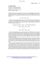
Figure 2 Flow curve of the austenitic steel X8CrNiMoNb16-16, described by Eqs. (13)
and (14).
Copyright 2004 by Marcel Dekker, Inc. All Rights Reserved.
The solution of this differential equation is
s ¼ C
1
þ C
2
e þ C

3
1 À expðÀC
4
eÞ½ ð14Þ
where C
1
is the yield stress, C
2
¼ kc=ðk
2
aGbÞ, C
3
¼ kð1 þ 2c=k
2
Þ=ðk
2
aGbÞ;
and C
4
¼ k
2
=2. This equation is identical with the empirical relation intro-
duced in Ref. [7]. It is found to give the optimum fit for the experimental
results of several materials (Fig. 2). However the determination of its para-
meter needs some more effort. It should be mentioned that also the empiri-
cal Swift relation given by Eq. (5) fits well the experimental data in this
strain range.
B. Influence of Strain Rate and Temperature
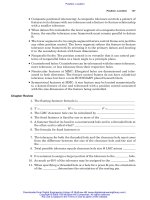
Figure 3a shows an example for the influence of increasing temperature on
the flow stress for given values of strain and strain rate [8]. Considering the

slope ds=dT, three different temperature ranges can be defined: (A) range of
low temperatures, between absolute zero and about 0.2 of the absolute melt-
ing point, where the influence of the temperature on the flow stress is great.
The material behavior is governed by thermally activated glide, (B) range of
intermediate temperatures between 0.2 and 0.5 of the absolute melting tem-
perature. Only a slight influence of strain rate and temperature on the flow
stress is usually observed in this range, and (C) range of temperatures higher
than 0.5T
m
in which the flow stress depends highly on the temperatures
because of the dominance of diffusion-controlled deformation processes.
The influence of the strain rate variation [9] is represented in Fig. 3b.
Three different strain rate ranges can also be recognized according to the
Figure 3 (a) Temperature influence on the yield stress of NiCr22Co12Mo9 at
_
ee ¼ 3 Â10
À4
sec
À1
[8]. (b) Influence of stain rate on shear yield stress of mild steel [9].
Copyright 2004 by Marcel Dekker, Inc. All Rights Reserved.
variation of @s=@ ln
_
ee: (I) range of low strain rates with only a slight influ-
ence of the strain rate due to athermal glide processes, (II) range of inter-
mediate and high strain rates with relatively high strain rate sensitivity
due to thermal activated glide mechanisms, and (III) range of very high
strain rates where internal damping processes dominate and a very high
strain rate sensitivity is observed. The boundary between the ranges (I)
and (II) depends on the temperature. Overviews concerning the mechanical

behavior under high strain rates are represented, e.g. in Refs. [10,11].
To estimate the mechanical behavior over wide ranges of strain rate
and temperature, constitutive equations must be established taking the time
dependent material behavior into consideration. A visco-plastic behavior is
often assumed by using, for example, the Perzyna equation [13]
_
ee
ij
¼
_
SS
ij
2m
þ
1 À 2v
2E
_
ss
kk
d
ij
þ 2ghFðFÞi
@f
@s
ij
ð15Þ
where m is the shear modulus, f is square root of the second invariant of the
stress deviator S
ij
and F ¼ (f=k) À1 is the relative difference between f and

the shear flow stress k ¼ s
F
=
ffiffiffi
3
p
. The function FðFÞ is often estimated using
simple rheological models assuming FðFÞ¼F and leading to linear relation
of the type s ¼ s
F
ðeÞþZ
_
ee which is acceptable for metals only at strain rates
>10
3
sec
À1
.
1. Empirical Relations
Different empirical relations could be implemented in Eq. (15). With
FðFÞ¼expðF =aÞÀ1 or FðFÞ¼F
1=m
, the corresponding relations between
stress and stress rate in the uniaxial case are identical with the empirical rela-
tions introduced 1909 by Ludwik [14]
s ¼ s
F
ðe; TÞ 1 þa lnð1 þ
_
ee=aÞ½ ð16Þ

s ¼ s
F
ðe; TÞ 1 þð
_
ee=a
Ã
Þ
m
½ð17Þ
The influence of temperature on the flow stress is also described by dif-
ferent relations of the type s ¼ sðe;
_
eeÞf ðT=T
m
Þ where T
m
is the absolute
melting point of the material, such as
s ¼ s
0
ðe;
_
eeÞexp ÀbT=T
m
½ ð18Þ
or according to Ref. [15]
s ¼ s
0
ðe;
_

eeÞ 1 ÀðT=T
m
Þ
v
½ ð19Þ
Copyright 2004 by Marcel Dekker, Inc. All Rights Reserved.
On applying such empirical relations, the flow stress is usually
represented by s ¼ f
t
ðeÞf
2
ð
_
eeÞf
3
ðTÞ as a product of three separate func-
tions of strain, strain rate and temperature. This is a rough approxima-
tion especially in the case of moderate strain rates of
_
ee < 10
3
sec
À1
.
However, the basic problem is that nearly all the parameters of these
empirical equations can only be regarded as constants only within rela-
tively small ranges of e,
_
ee, and T. The determination of the functional
behavior of the parameters requires a great number of experiments.

Therefore, constitutive equations based on structure-mechanical models
are gaining increasing interest as they can improve the description of
the mechanical behavior in wider ranges of strain rates and temperature
and may, if carefully used, allow for the extrapolation of the determined
relations.
2. Structure-Mechanical Models
The macroscopic plastic strain rate of a metal that results from the accumu-
lation of sub-microscopic slip events caused by the dislocation motion is
given by
_
ee ¼ br
m
v=M
T
ð20Þ
In this equation, the Burger vector b and the Taylor factor M
T
are
constants for a given material whereas the mobile dislocation density r
m
is mainly a function of strain. The relation between the dislocation velocity
v and the stress was experimentally determined for several materials [16]. It
can be represented in the range of low stresses by a power law
v ¼ v
0
ðs=s
0
Þ
N
. At very high stresses, the dislocation velocity approaches

asymptotically the shear wave velocity c
T
and s ¼ av
n
=
ffiffiffiffiffiffiffiffiffiffiffiffiffiffiffiffiffiffiffiffiffiffiffi
1 Àðv=c
T
Þ
2
q
.
3. Athermal Deformation Processes
In the range of intermediate temperatures and low strain rates (combined
ranges B and I), and at relatively low temperatures, i.e., less than 0.3 of
the absolute melting point T
m
, the influence of strain rate and temperature
depends on the
_
ee-range of the deformation process.
Below a specific value of the strain rate, that depends on tempera-
ture, only a slight influence of strain rate and temperature on the flow
stress is observed. In this region I, athermal deformation processes are
dominant, in which the dislocation motion is influenced by internal long
range stress fields induced by such barriers as grain boundaries, precipi-
tations, and second phases. The flow stress varies with temperature in the
Copyright 2004 by Marcel Dekker, Inc. All Rights Reserved.
same way as the modulus of elasticity. The influence of strain rate can be
described by

s ¼ C
EðTÞ
EðT
0
Þ
_
ee
m
ð21Þ
where E is the modulus of elasticity and m is of the order of magnitude
of 0.01.
4. Thermally Activated Deformation
In the ranges of low temperatures (A) and intermediate to high strain rates
(II), the dislocation motion is increasingly influenced by the short range
stress fields induced by barriers like forest dislocations and solute atom
groups in fcc-materials or by the periodic lattice potential (Peierls-stress)
in bcc materials. If the applied stress is high enough, these barriers can
immediately be overcome. At lower stresses, a waiting time Dt
w
is required
until the thermal fluctuations can help to overcome the barrier. A part of the
dislocation line becomes free to run, in the average, a distance s
Ã
until it
reaches the next barrier within an additional time interval Dt
m
. The mean
dislocation velocity is given by v ¼ s
Ã
=ðDt

w
þ Dt
m
Þ.
The waiting time Dt
w
equals the reciprocal value of the frequency
n of the overcoming attempts. If the strain rate is lower than ca. 10
3
sec
À1
, it can be assumed that Dt
w
4 Dt
m
. The relation between strain rate
and stress is then given by
_
ee ¼
_
ee
0
ðeÞ exp ÀDG=kT½where
_
ee
0
¼
br
m
n

0
s
Ã
=M
T
. The activated free enthalpy DG depends on the difference
s
Ã
¼ s À s
a
between the applied stress and the athermal stress according
to kT lnð
_
ee
0
=
_
eeÞ¼DG ¼ DG
0
À
R
V
Ã
ds
Ã
where V
Ã
¼ bl
Ã
s

Ã
=M
T
is the
reduced activation volume.
For given stress and strain, the value of T ln ð
_
ee
Ã
=
_
eeÞ is constant for all
temperatures and also for all strain rate values between
_
ee
0
exp½ÀDG
0
=
ðkTÞ and
_
ee
0
. This means that the increase of stress at constant strain with
decreasing temperature or with increasing strain rates is the same, as long
as the values of DG ¼ kT lnð
_
ee
Ã
=

_
eeÞ are equal in both cases.
Depending upon the formulation of the function V
Ã
ðs
Ã
Þ; different
relations for
_
ee ¼
_
ee
0
ðsÞ were proposed in Refs. [17–21]. The most
common are the relation introduced by Vo
¨
hringer [19,20] and by Kocks
et al. [21]
_
ee ¼
_
ee
0
ðeÞ exp À
DG
0
kT
1 À
s À s
a

s
0
À s
a

p

q

ð22Þ
Copyright 2004 by Marcel Dekker, Inc. All Rights Reserved.
and that by Zerilli and Armstrong [22,23]
s À s
a
¼
DG
0
V
Ã
0
exp À b
0
þ
k
DG
0
ln
_
ee
0

_
ee

T

ð23Þ
5. Transition to Linear Viscous Behavior
At strain rates higher than some 10
3
sec
À1
, the stress is high enough to the
extent that Dt
w
vanishes. Only the motion time Dt
m
is to be considered. The
dislocation run with high velocity throughout the lattice and damping
effects dominate. The dislocation velocity v ¼ s
Ã
=Dt
m
can then be given by
v ¼ bðt Àt
h
Þ=B according to Ref. [24]. The flow stress follows the relation
s ¼ s
h
ðe; TÞþZ
_

ee ð24Þ
with Z ¼ M
T
B=ðb
2
N
m
Þ. This relation is validated experimentally in Ref. [9]
as well as by Sakino and Shiori [25], as shown in Fig. 4a. A continuous tran-
sition takes place, when the strain rate is increased from the thermal activa-
tion range (II) to the damping range (III). This can be described in two
different ways: regarding the dislocation velocity to be equal to
v ¼ s
Ã
=ðDt
w
þ Dt
m
Þ, the strain rate can be represented by
_
ee ¼
_
ee
0
exp
DG
0
kT
1 À
s À s

a
s
0
À s
a

p

q

þ
x
s À s
h

À1
ð25Þ
where x is a function of strain. Alternatively, the continuous transition can
be described by an additive approximation. The stress is regarded to be the
sum of the athermal, the thermal activated and the drag stress components.
According to this approximation, s % s
a
þ s
th
þ Z
_
ee where s
th
is the thermal
activated component of stress determined from Eq. (22) or (23).

6. Diffusion-Controlled Deformation
In the range of high temperatures (C), the deformation is governed by strain
hardening and diffusion-controlled recovery processes
_
ee ¼
_
ee
0
s
G

n
exp À
Q
1
RT

ð26Þ
At very high temperatures and low stresses
_
ee
d;e
¼ 14
sO
kT
1
d
2
D
v

1 þ
pdD
B
dD
v

ð27Þ
Copyright 2004 by Marcel Dekker, Inc. All Rights Reserved.
C. Material Laws for Wide Ranges of Temperatures
and Strain Rates
Material laws that describe the flow behavior over very wide ranges of tem-
peratures and strain rates are needed for the simulation of several deforma-
tion processes, such as high-speed metal cutting. In this case, different
physical mechanisms have to be coupled by a transition function. Fig. 5
shows the dependence on the stre ss with the strain rate at different tempera-
tures for a constant strain. Three main mechanisms can be distinguished: (a)
diffusion-controlled creep processes with
_
ee
cr
/ s
NðT Þ
in the region (1) of low
strain rates and high temperatures, (b) dislocation glide plasticity with
s /
_
ee
mðTÞ
pl
in the region (2) of intermediate temperatures and strain rates,

and (c) viscous damping mechanism with s ¼ s
G
þ Zð
_
ee À
_
ee
G
Þ in the region
of very high strain rates
_
ee > 1000 sec
À1
in the region (3).
1. Visco-plastic Material Law
For a continuous description over the different ranges, the strain rates have
to be combined [27] to obtain
_
ee ¼ 1 ÀMðÞ
_
ee
kr
þ
_
ee
pl

þ M
_
ee

damping
ð28Þ
with the transition function M ¼ 1 À exp½Àð
_
ee=
_
ee
G
Þ
m
. The complete strain
rate range can be described by
_
ee ¼ 1 ÀMðÞ
s
s
0
T; eðÞ

NTðÞ
þ
s
s
H
T; eðÞ

1=mTðÞ
!
_
ee

Ã
þ M
s À s
G
T; eðÞ
Z
þ
_
ee
G
T; eðÞ

ð29Þ
with
_
ee
Ã
¼ 1 sec
À1
. The parameters and functions s
0
(T, e), s
H
(T, e), m(T),
N(T), and Z have to be determined by curve fitting in the individual regions
(1)–(3), whereas the parameters s
G
and
_
ee

G
are determined requiring that the
derivative @s=@
_
ee follows a continuous function in the transition region:
s
G
¼ s
H
ð
_
ee
G
=
_
ee
Ã
Þ
m
and
_
ee
G
¼ðms
H
=ZÞ
1=ð1ÀmÞ
. The values of the parameter
used are given in Ref. [28].
An exception of the rule of the reduction of flow stress with increasing

temperature is the influence of dynamic strain hardening observed in ferritic
steel at temperatures between 2008C and 4008C, where the flow stress
increases towards a local maximum. It is caused by the interaction between
moving dislocations and diffusing interstitial atoms . The additional stress
can be described by Ds ¼ að
_
eeÞ exp½ÀfðT Àbð
_
eeÞÞ=cð
_
eeÞg
2
, With this addi-
tional term, the dependence of flow stress of steel Ck45 (AISI 1045) on tem-
perature and strain rate is determined [28] and represented in Fig. 6.
Copyright 2004 by Marcel Dekker, Inc. All Rights Reserved.
2. Adiabatic Softening
Flow curves determined in the range of high strain rates are almost adiabatic,
since the deformation time is too short to allow heat transfer. The major
part of the deformation energy is transformed to heat while the rest is
consumed by the material to cover the increase to internal energy due
to dislocation multiplication and metallurgical changes. On strain increase
by de, the temperature increases according to
dT ¼ k
0:9
rc
s de ð30aÞ
where the factor 0.9 is the fraction of the deformation work transformed to
heat, s is the current value of the flow stress which is already influen ced by
the previous temperature rise and k is the fraction of energy remaining in the

deformation zone. At low strain rate, there is enough time for heat transfers
out of the deformation zone and the temperature increase is negligible. In
this case, k ¼ 0. On the other hand, the deformation process is almost adia-
batic at high strain rate and k ¼ 1. A continuous transition from the isother-
mal deformation under quasi-static loading to the adiabatic behavior under
dynamic loading can be achieved considering k as a function of strain rate in
the form.
Figure 7 Quasi-static and adiabatic flow curves of unalloyed fine grained steel.
Copyright 2004 by Marcel Dekker, Inc. All Rights Reserved.
kð
_
eeÞ¼
1
3
þ
4
3p
arctan
_
ee
_
ee
ad
À 1

ð30bÞ
The transition strain rate
_
ee
ad

depends on the thermal properties of the
material. If the temperature of the surroundings is the room temperature,
_
ee
ad
is around 10
þ1
sec
À1
.
As the flow stress usually decreases with increasing temperature, the
flow curve shows a maximum (Fig. 7). A thermally induced mechanical
instability can take place leading to a concentration of deformation, a
localization of heat and even to the formation of shear bands.
An overview of different criteria for the thermally induced mechanical
instability is presented in Ref. [29]. The adiabatic flow curve can be deter-
mined numerically for an arbitrary function sðe;
_
ee; TÞ for the shear stress
which has been determined in isothermal deformation tests. In order to
obtain a closed-form analytical solution demonstrating the adiabatic flow
behavior, the simple stress–temperature relation s ¼ s
iso
ðe;
_
eeÞCðDTÞ can
be used [30,31]. In this case, the change of temperature can simply be deter-
mined by separation of variables and integration. For example,
s ¼ s
iso

ðe;
_
eeÞ 1 À m
T À T
0
T
m

; s ¼ s
iso
exp À
0:9km
rcT
m
Z
s
iso
de

ð31Þ
s ¼ s
iso
ðe;
_
eeÞ exp Àb
T ÀT
0
T
m


; s ¼ s
iso
1 þ
0:9kb
rcT
m
Z
s
iso
de

À1
ð32Þ
T
m
is the absolute melting point of the material,

rr and

cc are the mean values
of density and specific heat in the temperature range considered. Around
room temperature, the product rc lies between 2 and 4 MPa=K for most
of the materials. For a rough approximation, it can be assumed that
(rcT
m
=0.9) % 3T
m
in MPa using T
m
in K.

Many experimental investigations e.g. Ref. [32] were carried out in
order to determine the temperature dependence of the flow stress. Up to a
homologous temperature of 0.6, the stress–temperature relation can be
described better by Eq. (35) than by Eq. (34), showing values of b between
1 and 4. Therefore, only Eq. (35) will be considered in the following discus-
sion. If the isothermal stress can be simply described by
s
iso
% Ke
n
Fð
_
eeÞð33Þ
the flow stress, determined in an adiabatic test with constant
_
ee, is then
given by
Copyright 2004 by Marcel Dekker, Inc. All Rights Reserved.
s
ad
¼ Ke
n
Fð
_
eeÞ 1 þ
ka
ð1 þ nÞT
m
Ke
1þn

Fð
_
eeÞ

À1
ð34Þ
where a ¼ 0:9b=ð

rr

ccÞ. The parameter a can be considered as approximately
constant represented by its mean value over the deformation process which
is of the order of magnitude of 1 K=MPa. The flow curve shows a maximum
s
max
at the critical strain e
c
, where
e
c
¼
nð1 þ nÞT
m
k aKFð
_
eeÞ

1=ð1þnÞ
; s
max

¼
KFð
_
eeÞ
1 þ n
nð1 þ nÞT
m
k aKFð
_
eeÞ

n=ð1þnÞ
ð35Þ
and the parameters K and a can be estimated by
K ¼
1 þ n
Fð
_
eeÞ
s
max
e
n
c
; k a ¼
nT
m
s
max
e

c
ð36Þ
the remaining unknown parameter n can be determined by fitting the curve
the adiabatic flow curve [12].
Similar to the process of neck formation in a tensile specimen, the exis-
tence of a stress maximum leads to mechanical instability. Especially after
reaching the stress maximum, a great part of the specimen is unloaded elas-
tically causing further deformation localization. In dynamic torsion tests,
the deformation localization leads to a heat concentration and hence a
higher local temperature rise and a high shear strain concentration. Coffey
and Armstrong [33] introduced a global temperature localization factor
which is the ratio of the plastic zone volume to the total specimen volume.
The influence of inhomogeneity on the strain distribution has been demon-
strated by using a simple model [34] which represents the torsion specimen
by two slices, a reference one and another slice with slight deviations in
strength or dimensions. Furthermore, the deformation localization could
be traced during the torsion test by observing the deformation of grid lines
on the specimen surface by means of high-speed photography [35,36].
The influence of adiabatic softening can be illustrated in the case of
compression test at high strain rates.
Due to friction between the cylindrical specimen and the loading
tools, a compression specimen becomes a barrel form during the test. In
an etched cross-section of a quasi-statically tested specimen, two conical
zones of restricted deformations can often be recognized after quasi-static
upsetting. The deformed geometry is symmetrical about the midplane
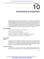
(Fig. 8). An FE-simulation is carried out for a compression test with
_
ee¼
0.001 sec
À1

considering stain hardening according to Eq. (8) and friction
at the upper and lower surfaces by a coefficient m ¼ 0.1. The computa-
tional results indicate that the maximum values of equivalent stress as well
Copyright 2004 by Marcel Dekker, Inc. All Rights Reserved.
Figure 9 Quasi-static compression test on cylind rical specimens with
_
ee ¼
0:001 sec
À1
. (a) Etched section of a SMnPb-steel. (b) Distribution of Mises’ stress.
(c) Distribution of the equivalent plastic.
Copyright 2004 by Marcel Dekker, Inc. All Rights Reserved.
(Fig. 12a). The combination of experiment and finite-element simulation
allows examining the possibility of extrapolation of materials laws to the
range of very high strains and strain rates [28]. In addition, valuable infor-
mation can be obtained for the optimization of the width B in shear
Figure 10 Etched longitudinal section of a cylindrical compression specimen of
Armco iron loaded dynamically (
_
ee ¼ 5000 sec
À1
).
Figure 11 Distribution of Mises’ stress and equivalent plastic strain in a
compression specimen after dynamic test with
_
ee ¼ 5000 sec
À1
, friction coefficient
m ¼ 0.1.
Copyright 2004 by Marcel Dekker, Inc. All Rights Reserved.

Figure 13 Distribution of the equivalent stress and the equivalent stress in the
shear zone of a hat-shaped specimen [28]. (a) Equivalent strain. (b) Equivalent stress
in MPa according to von Mises.
Copyright 2004 by Marcel Dekker, Inc. All Rights Reserved.
displacement–time function of the upper surface is applied to upper the
nodes. In order to reduce the total number of elements, the lower die is idea-
lized using the so-called infinite elements.
The material law is determined in compression tests at different
temperatures with strain rates up to 7500 sec
À1
. As discussed above, one
can assume a linear viscous behavior according to s ¼ s
h
ðeÞþZ
_
ee, when
_
ee > 2000 sec
À1
and the damping mechanism dominates. The simulation
should examine the accuracy of the reproduction of the force–displacement
curves determined experimentally for this geometry.
The distributions of the von Mises equivalent stress and equivalent
strain, represented in Fig. 13, show a great non-uniformity. High strain con-
centrations exist at the two diagonally opposite corners of the deformation
zone. In these regions, the strain rate is so high that the influence of adiabatic
softening is more than compensated and high stress values are determined
there.
Examples for the force–displacement curves determined experimen-
tally and computed by the FEM are shown in Fig. 14 for different values

of the shear zone width B. The deviation of the computed curves from the
experimental ones is relatively small. Therefore, it can be assumed that
the material law determined in the range of high strain rates
_
ee > 2000 sec
À1
Figure 14 Force–displacement curves of the hat specimen. Markers: experimental
results, curves: FE simulation. (From Ref. 28.)
Copyright 2004 by Marcel Dekker, Inc. All Rights Reserved.
can be extrapolated to much higher strain rates assuming the dominance of
the viscous damping mechanism according to Eq. (24). This result is consis-
tent with the experimental results of Sakino and Shiori (Fig. 4a).
Such material laws allow the simulation of different metal forming as
well as metal cutting processes. They can be validated by high-speed metal
cutting tests [38]. Structural damage during high rate tensile deformation
can be accounted for by introducing a damage function [39].
II. CYCLIC DEFORMATION BEHAVIOR
A. Phenomenological Approach
If a specimen is extended with a constant strain rate
_
ee
0
, the stress increases
first according to Hooke’s law of elasticity till the elastic limit is reached.
Then, a plastic deformation begins accompanied with a non-linear harden-
ing. After reaching an arbitrary total strain e
1tot
¼ e
1el
þ e

1pl
, the strain rate
changes to (À
_
ee
0
). At first, the material is unloaded elastically and is then
compressed until a total strain of (Àe
1tot
), as represented in Fig. 15.
It can be clearly observed that the plastic compression begins at an
elastic limit R
=
e
, whose absolute value much smaller than the initial value
Figure 15 Stress–strain diagram of an experiment with a change of the loading
direction.
Copyright 2004 by Marcel Dekker, Inc. All Rights Reserved.
R
e
. In general, it can be stated that a previous tensile deformation reduces
the compression elastic limit. Also, a compression deformation reduces
the subsequent elastic limit under tension. This phenomenon,known as
Bauschinger effect, is characteristic for the behavior of the material under
cyclic loading in the low cycle fatigue range. With further cyclic loading,
the stress range increases usually due to strain hardening (Fig. 16). If the
material is highly pre-deformed or hardened, a cyclic softening takes place
and the stress range decreases with increasing number of cycles.
The rate of change of the stress range Ds decreases with the number of
cycles and approaches a stationary value and the hysteresis loop remains

unchanged.
The strain hardening phenomena under cyclic loading can be classified
in two terms:
(a) Isotropic deformation resistance s
F
, that includes the yield point
as well as the isotropic change of the flow stress. It increases (or
decreases) monotonically with the number of cycles, depending
upon the specific plastic deformation work
R
s de, or on the
accumulated plastic strain
P
dejj. Its variation with strain can be
considered as a result of the increase of the density of immobile
Figure 16 Stress–strain diagram of an austenitic steel under cyclic loading with a
constant range of the total strain of De ¼ 0:0066 at 6508C.
Copyright 2004 by Marcel Dekker, Inc. All Rights Reserved.
dislocation with an additional influence of the changing micro-
scopic residual stress state.
(b) Kinematic hardening or internal back stress s
i
that depends on
the direction of the deformation and the loading history and
accounts for the Bauschinger effect. It may result from the
reversible interactions of mobile dislocations with obstacles, such
as in the cases of pile ups or bowing between particles.
Figure 17 shows the influence of these stress parts in the biaxial case
on the form of the Mises-ellipse. The isotropic hardening leads to an equal
increase of the ellipse in all directions, while the kinematic hardening shifts

the ellipse in the loading direction. Usually, both of these hardening types
are to be expected during plastic deformation.
During uniaxial cyclic deformation, the influence of the strain rate can
be considered in two ways:
s À s
i
ðÞ
2
¼ s
2
F
Fð
_
ee
pl
Þð37aÞ
s À s
i
ðÞ
2
¼ s
F
þ Cð
_
ee
pl
Þ

2
ð37bÞ

If the direction of the strain rate, and hence its sign, is suddenly chan-
ged, the sign of the isotropic material resistance s
F
changes at once. In con-
trast, the value of internal back stress s
i
changes gradually with increasing
deformation approaching asymptotically a stationary value s
is
with the
same sign as the strain rate.
In the first cycle, the stress equals s
F0
þ s
i0
, at the beginning of the plas-
tic deformation where s
i0
is approximately equal to 0 for annealed materials.
With increasing strain, both of s
F
and s
i
increase approaching the stationary
Figure 17 Mises’ ellipse after: (a) isotropic hardening, (b) kinematic hardening,
and (c) mixed mode hardening.
Copyright 2004 by Marcel Dekker, Inc. All Rights Reserved.
values s
F1
and s

is
. On reaching the maximum strain of De
tot
=2, the maxi-
mum stress is given by s
max1
¼ s
F1
þ s
i1
. If the loading direction is changed
from tension to compression, the isotropic material resistance changes from
(þs
F1
)to(Às
F1
) at once. The material is first unloaded and the stress drops
by the amount of s
F1
. With further reduction of length, plastic compression
start when the stress is reduced by 2s
F1
. During this short time, the internal
back stress s
i
remains unchanged at the value s
i1
. After the beginning of plas-
tic compression, it starts to decrease gradually approaching a new stationary
value ðÀs

is
Þ that corresponds to the new strain rate of (À
_
ee ).
Each time when the strain rate changes from (þ
_
ee)to(À
_
ee) in an arbi-
trary cycle, the stress drops during the elastic deformation by Ds
F
¼ 2s
F
and then gradually by Ds
i
during the plastic deformation of the half cycle.
On the next reverse (À
_
ee)to(þ
_
ee), a stress decreases first by Ds
F
and then gra-
dually by Ds
i
. The stress ranges is Ds ¼ Ds
F
þ Ds
i
. The maximum and the

minimum stress s
max
¼ s
F
þ Ds
i
=2 and s
min
¼Às
F
À Ds
i
=2.
The range Ds
F
is defined as the difference between the maximum stress
and the elastic limit in the subsequent compression phase. Especially in cyc-
lic deformation, it is rather difficult to exactly determine the elastic limit,
i.e., the transition point between the elastic and plastic deformation ranges
because this transition is almost gradual. However, this point can be easily
estimated if the hysteresis loop (Fig. 18a) is differentiated and ds=de
tot
is
represented as a function of s (Fig. 18b). Starting at minimum stress (point
1), the slope of the curve remains approximately constant and equals the
modulus of elasticity till point 2 is reached. Then the slope decreases to a
Figure 18 (a) Hysteresis loop, and (b) the derivative with respect to the total strain
as a function of the stress.
Copyright 2004 by Marcel Dekker, Inc. All Rights Reserved.
relatively low value at point 3 of the maximum stress. The stress–strain

curve rotates to point 4 of maximum strain. The slope decreases to À1,
changes to þ1 and decreases again to the value of the modulus of elasticity.
This value should remain unchanged till point 5, where plastic compression
begins and the slope decreases again till reaching point 6. Between point 6
(minimum stress) and point 1 (minimum strain), the value of slope changes
to þ1 then to þ1 and decreases to the value of the modus of elasticity. The
relation between ds=de
tot
and s can be linearized in the plastic ranges
between the points 2 and 3 as well as between points 5 and 6. The intersec-
tion of these linear relations with the elastic relation ds=de
tot
¼ E defines the
value of range Ds
F
of the isotropic material resistance. The range of the
internal back stress is the defined by Ds
i
¼ Ds þ Ds
F
:
Repeating the procedure represented in Fig. 18 for the different cycles,
one obtains Fig. 19a. For each half cycle, the value of Ds
F
and the linear
relation between ds=de and s can be determined.
The isotropic component s
F
as well varies monotonically and continu-
ously with increasing number of cycles. However, it can be assumed that its

value is constant within arbitrary half cycles and changes only at the begin-
ning of the next one, if the total number of cycles is great enough. In this case
ds
i
de
¼
ds
de
ð38Þ
within each half cycle. The linear relation
ds
i
de
tot
¼ E 1 À
s
i
À s
i0
s
is
À s
i0

ð39Þ
can be written for the internal back stress as well. The stationary value s
is
varies with the number of cycles.
The isotropic material resistance s
F

as well as the stationary value s
is
of the internal back stress s
i
are represented in Fig. 19b as functions of the
accumulated strain.
These relations may be described by
s
F
¼ s
F0
þ s
F1
À s
F0
ðÞ1 À exp ÀC
F
e
acc
ðÞ½ ð40Þ
s
is
¼ s
is0
þ s
is1
À s
is0
ðÞ
1 À exp ÀC

i
e
acc
ðÞ½
ð41Þ
yielding the evolution equations
ds
F
de
acc
¼ C
F
s
Fs
À s
F
ðÞ ð42Þ
ds
is
de
acc
¼ C
i
s
is1
À s
is
ðÞ ð43Þ
Copyright 2004 by Marcel Dekker, Inc. All Rights Reserved.
achieved by considering two internal variables for the internal back stress

instead of only one as considered here [40].
With de
pl
¼ de
tot
À ds
i
=E, the derivative of the internal back stress
with respect to the plastic strain can be obtained from Eq. (39) as
ds
i
de
pl
¼ E
s
is
À s
i0
s
i
À s
i0
À 1

ð44Þ
A comparison of this relation with the experimental results is repre-
sented in Fig. 20b.
B. Constitutive Equation of Cyclic Behavior
In contrast to these experimental facts, serious simplifications are usually
made to reduce the number of the material parameters involved in

computation. The hyperbolic function of Eq. (8) is simply linearized
yielding
ds
i
de
pl
¼ C À gs
i
ð45Þ
Figure 20 Relation between stress derivative and internal back stress s
i
. (a)
Derivative with respect to the total stress. (b) Derivative with respect to plastic strain.
Copyright 2004 by Marcel Dekker, Inc. All Rights Reserved.
where C and g are material constants. The stationary value s
is
is considered
constant assuming that the material follows the Masing-rule and Eq. (5) is
reduced to
s
is
¼ C=g ð46Þ
Lemaitre and Chaboche [41,42] introduced a non-linear isotropic=
kinematic hardening model, which provides predictions that are near to
the experimental evidence. This model is applicable for isotropic incom-
pressible materials. The yield surface is defined by the function
F ¼ fðs
ij
À X
ij

ÞÀs
0
¼ 0 ð47Þ
where s
0
is the yield stress that is equivalent to the isotropic material resis-
tance s
F
and X
ij
is the tensor of the internal back stress denoted s
is
in the
uniaxial case. The function f ðs
ij
À X
ij
Þ equals the equivalent Mises stress
when the back stress X is taken into consideration:
f ¼
ffiffiffiffiffiffiffiffiffiffiffiffiffiffiffiffiffiffiffiffiffiffiffiffiffiffiffiffiffiffiffiffiffiffiffiffiffiffiffiffiffiffiffi
3
2
ðs
0
ij
À X
0
ij
Þðs

0
ij
À X
0
ij
Þ
r
ð48Þ
where s
0
ij
is the deviatoric stress tensor and is the X
0
ij
deviatoric part of the
back stress tensor. The associated plastic flow is given by
_
ee
pl
ij
¼
@F
@s
ij

_
ee
_
ee
pl

¼
3
2
ðs
0
ij
À X
0
ij
Þ
f

_
ee
_
ee
pl
ð49Þ
where
_
ee
pl
represents the rate of plastic flow and
_

ee

ee
pl
is the equivalent plastic

strain rate

_
ee
_
ee
pl
¼
ffiffiffiffiffiffiffiffiffiffiffiffiffi
2
3
_
ee
pl
ij
_
ee
pl
ij
r
ð50Þ
The size of the elastic range, s
0
, is a function of the equivalent plastic
strain

ee
pl
and the temperature. For a constant temperature, it is written simi-
lar to Eq. (40) as

s
0
¼ s
0
þ Q
1
1 À expðÀb

ee
pl
Þ



ð51Þ
where s
0
j
is the yield surface size at zero plastic strain, and Q
1
and b are
additional material parameters that must be determined from cyclic
experiment.
Copyright 2004 by Marcel Dekker, Inc. All Rights Reserved.
The evolution of the kinematic component of the model, when tem-
perature and field variable are neglected, is defined as
_
XX
ij
¼

2
3
C
_
ee
pl
ij
À X
ij

_
ee
_
ee
pl
¼ C
s
0
ij
À X
0
ij
s
0
À gX
ij


_
ee

_
ee
pl
ð52Þ
where C and g are material parameters.
C. Application to Life Assessment
The assessment of the fatigue life under cyclic elasto-plastic deformation
requires an accurate determination of the strain ranges of the individual
loading cycles in the region of maximum local deformation. For this reason,
FE simulation is often needed especially when the analytical solutions are
not available or when they include unacceptable simplifications.
For example, the fatigue life of notched machine parts is often predicted
using approximation formulas [43–45] that have been driven using the Neu-
ber rule [46]. However, the accuracy of these methods remains lower than that
of the inelastic FE analysis, when adequate materials lows are implemented.
Figure 21a illustrates the distribution of the axial stress s
xx
in a
notched 3-point bending specimen. The mesh is built of three-dimensional
continuum solid elements. Around the notch, a refined mesh is chosen so
that the critical zone at notch root would cover several elements. The mate-
rial considered is the AlZnMgCu alloy AA7075. The material parameters
determined in uniaxial cyclic experiments are: sj
0
¼310 MPa, Q ¼ 75 MPa,
b ¼ 36.6, C ¼ 14,844 MPa and g ¼ 86.3. As a loading condition, a line load
with a total compressive force F is applied at the midlength of the upper sur-
face. The force follows a sinusoidal time function with F
min
=F

max
¼ 0:1. The
specimen is supported at two parallel lines on the lower surface with a span
width of 80 mm. The computational results of the local strain components at
notch root are represented in Fig. 21b as functions of time.
For an arbitrary loading cycle, the time functions e
ij
ðtÞ are used to
determine an equivalent strain range D

ee for the cycle according to different
approaches [47–52].
With an additional damage accumulation rule, a representative peri-
odically repeated strain range can be computed which should lead to the
same fatigue life.
Experimentally, fatigue life is determined as the number of cycles, at
which a technically detectable crack is initiated. Often, a direct current
potential drop system [53,54] is used to determine the potential drop across
the notch as time function. This is then converted to a relation between
crack length and number of cycles to initiate cracks.
Copyright 2004 by Marcel Dekker, Inc. All Rights Reserved.