Strength Analysis in Geomechanics Part 5 potx
Bạn đang xem bản rút gọn của tài liệu. Xem và tải ngay bản đầy đủ của tài liệu tại đây (423.01 KB, 20 trang )
68 3 Some Elastic Solutions
P
x
y
τ
e
= const
u
y
σ
y
Fig. 3.19. Pressure of punch
3.2.9 Stresses and Displacements Under Plane Punch
M. Sadowski solved this problem (Fig. 3.19) using the analogy method /20/.
Replacing in the second relation (3.8) Q, ζ,w
(ζ)byP,z,2iF
(z) respectively
we receive
F
(z) = −P/2π
l
2
− z
2
, F(z) = −(Pi/2π)ln(z+
z
2
− l
2
)+2Gu
o
. (3.95)
We can easily notice that this result can be got from the first expres-
sion (3.84) after the consequent replacement of z, l, σ, by 1/z, 1/l, −Pi/πl
respectively.
With a help of (3.82), (3.83) we find a distribution of stresses (broken line
for σ
y
in Fig. 3.19) and displacement u
y
(solid curves outside the punch) at
y=0atx< l, x > l respectively as
u
y
=u
o
, τ
xy
=0, σ
x
= σ
y
= −P/π
l
2
− x
2
, (3.96)
σ
x
= σ
y
= τ
xy
=0, u
y
=u
o
− (P/2πG)(1 + κ)ln(x/l −
(x/l)
2
− 1). (3.97)
The computations show that diagram u
y
outside the punch is near to that
one for uniformly distributed load according to (3.51).
In a similar way as before we find with a help of (3.95), (3.82), (3.83) and
(2.65) in the asymptotic approach
σ
r
σ
θ
= −(P/π
√
2rl)(1 ± cos
2
(θ/2)) sin(θ/2),
τ
rθ
=(P/2π
√
2rl) sin θ sin(θ/2), τ
e
=(P/2π
√
2rl) sin θ,
(3.98)
u
θ
=u
1
− (P/πG)
r/2l(0.5(κ +1)−sin
2
(θ/2)) cos(θ/2),
u
r
=u
2
− (P/πG)
r/2l(0.5(κ − 1) + cos
2
(θ/2)) sin(θ/2)
(3.99)
where u
1
, u
2
– constants. It is easy to notice that τ
e
in this task differs from
that in the problem of crack (see the fourth relation (3.90)) by a constant
3.2 Plane Deformation 69
multiplier. The condition τ
e
= constant is shown by pointed line in the left
part of Fig. 3.19 under the edge of the punch and the plastic zone must have
this form.
3.2.10 General Relations for Transversal Shear
In this case we have on axis x condition σ
y
= 0 and from (3.68) we find after
some simple transformations
χ
(z) = −(2F
(z) + zF
(z)), χ(z) = −(F(z) + zF
(z)). (3.100)
Putting these expressions into (3.68), (3.69) we receive
σ
y
− σ
x
+2iτ
xy
= −4(F
(z) + iyF
(z)), (3.101)
2G(u
x
+iu
y
)=κF(z) + F(z) − 2iyF
(z). (3.102)
From (3.101) we have at y = 0
τ
xy
= −2ImF
(x
o
)
that is twice τ
y
-value in the problem of the longitudinal shear in (3.5) and we
can replace in the results of sub-chapter 3.1 w
(z) by 2F
(z).
3.2.11 Rupture Due to Crack in Transversal Shear
In this case (Fig. 3.20) τ
xy
(∞)=τ and we derive from (3.14)
F
(z) = −iτz/2
z
2
− l
2
, F(z) = −0.5iτ
z
2
− l
2
(3.103)
and according to (3.102) we find on axis x at x </l/ and x >/l/ respectively
τ
xy
=u
y
= σ
y
=0, σ
x
= −2τx/
l
2
− x
2
, u
x
= −τ((κ +1)/2G)
l
2
− x
2
,
σ
x
= σ
y
=u
x
=0, τ
xy
= τx/
x
2
− l
2
, u
y
=((κ −1)/2G)
x
2
− l
2
(3.104)
y
x
τ
τ
τ
τ
Fig. 3.20. Crack in transversal shear
70 3 Some Elastic Solutions
and by the Clapeyron’s theorem (3.17) as well as the energy balance
(1 + κ)πlτ
∗
2
dl/4G = 4γ
s
dl
we compute
τ
∗
=4
γ
s
/π(κ + 1)l. (3.105)
The same results can be received according to the asymptotic approach
and (3.102), (3.103) as
σ
r
= −(K
2
/
√
2πr)(2 −3cos
2
(θ/2)) sin(θ/2), σ
θ
= −3(K
2
/
√
2πr) cos
2
(θ/2) sin(θ/2),
τ
rθ
=(K
2
/
√
2rπ)(1 −3sin
2
(θ/2)) cos(θ/2), τ
e
=(K
2
/2
√
2πr)
√
1+3cos
2
θ,
(3.106)
u
r
u
θ
=(K
2
/2G)
r/2πx
(−κ +5− 6sin
2
(θ/2)) sin(θ/2)
(−κ − 5+6cos
2
(θ/2)) cos(θ/2).
(3.107)
Here K
2
= τ
√
πl – the stress intensity coefficient of the second crack task.
Further computation follows that one for a crack in tension and we find a
similar value (see also (3.93))
K
2
∗ =4
Gγ
s
/(κ + 1) (3.108)
and the strength condition
K
2
≤ K
2
∗ .
Diagrams σ
θ
/σ
yi
, σ
r
/σ
yi
, τ/σ
yi
at τ
e
= σ
yi
/2 as functions of θ are given
in Fig. 3.21 by solid, broken and interrupted by points lines 1 respectively.
3.2.12 Constant Displacement at Transversal Shear
Using the analogy mentioned above we have from (3.8) at ζ =z
F
(z) = −Q/2π
z
2
− l
2
, F(z) = 2Gu
o
−(Q/2π)ln(z/l+
(z/l)
2
− 1) (3.109)
0
0.5
−0.5
−1
0
0 30 60 90 120 150
θ
o
σ
θ
/σ
yi
σ
r
/σ
yi
τ/σ
yi
0
0
0
0
0
1
1
1
1
1
Fig. 3.21. Diagrams of stress distribution at crack ends in transversal shear
3.2 Plane Deformation 71
wherein Q is a resultant of τ
xy
at y = 0, −l < x < l. From (3.101), (3.102),
(3.109) we find on axis x at x </l/ and x >/l/ respectively
u
x
=u
o
, u
y
= σ
x
= σ
y
=0, τ
xy
=Q/π
l
2
− x
2
,
τ
xy
=u
y
= σ
y
=0, σ
x
= −2Q/π
x
2
− l
2
,
u
x
=u
o
− (Q/2πG)(κ +1)ln(x/l+
(x/l)
2
− 1).
In the asymptotic approach we receive similarly to (3.106), (3.107) as
σ
r
= −(Q/π
√
2rl)(3 cos
2
(θ/2) −1) cos(θ/2), σ
θ
= −3(Q/π
√
2rl) sin
2
(θ/2) cos(θ/2),
τ
rθ
=(Q/π
√
2rl)(3 sin
2
(θ/2) −2) sin(θ/2), τ
e
=(Q/2π
√
2rl)
1+3cos
2
θ, (3.110)
u
r
=u
1
− (Q/πG)
r/2l((κ +1)/2 − sin
2
(θ/2)) cos(θ/2),
u
θ
=u
2
− (Q/πG)
r/2l((κ − 1)/2 − 3cos
2
(θ/2)) sin(θ/2).
And we again can see that τ
e
in (3.106), (3.110) differ by a constant multiplier.
3.2.13 Inclined Crack in Tension
By a combination of the solutions in Sects. 3.2.7, 3.2.11 a strength of a body
with inclined crack in tension (Fig. 3.22) can be studied. Supposing according
to (2.72) σ =psin
2
β, τ =0.5p sin 2β and seeking in the end of the crack main
plane with θ = θ
∗
L. Kachanov found in /17/ relation
sin θ
∗
+(3cosθ
∗
− 1)cotβ = 0 (3.111)
according to which the crack must propagate in this direction. Some experi-
ments confirm it.
y
p
p
x
θ
*
β
Fig. 3.22. Inclined crack in tension
72 3 Some Elastic Solutions
3.3 Axisymmetric Problem and its Generalization
3.3.1 Sphere, Cylinder and Cone Under External and Internal
Pressure
For a sphere with internal a, current ρ and external b radii (Fig. 3.23) we use
equations (2.80) and the Hooke’s law (2.17) at σ
θ
= σ
χ
in the form
σ
θ
=E(ε
θ
+ νε
ρ
)/(1–ν−2ν
2
), σ
ρ
=E(ε
ρ
(1 −ν)+2νε
θ
)/(1 −ν−2ν
2
). (3.112)
Putting (2.81) into (3.112) and the result – in (2.80) we get on a differential
equation for u
ρ
≡ u
d
2
u/dρ
2
+2du/ρdρ–2u/ρ
2
=0
with an obvious integral
u=A/ρ
2
+Bρ. (3.113)
Now we determine strains from (2.80), stresses – by (3.112) and constants –
according to boundary conditions σ
ρ
(a) = −q, σ
ρ
(b) = −p. As a result we
have
σ
θ
=(qa
3
(2ρ
3
+b
3
)–pb
3
(2ρ
3
+a
3
))/2ρ
3
(b
3
a
3
),
σ
ρ
=(qa
3
(ρ
3
–b
3
)+pb
3
(a
3
− ρ
3
))/ρ
3
(b
3
− a
3
).
(3.114)
The strains and the displacements can be found according to the Hooke’s law
and expressions (2.80).
In a similar way the stress distribution in a tube can be analysed. To
change the method we use here potential function Φ (see Sect. 2.4.3) since the
problem is a plane one. The biharmonic equation (2.74) in this case becomes
d(rd(d(rdΦ/dr))/rdr)/dr)/rdr = 0
a
b
q
p
ρ
Fig. 3.23. Sphere under internal and external pressure
3.3 Axisymmetric Problem and its Generalization 73
p
λ
χ
ρ
Ψ
q
O
Fig. 3.24. Cone under external and internal pressure
with a very simple solution that with a help of (2.75) and boundary conditions
like that for the sphere (with replacement in them ρ by r) gives
σ
r
=(a
2
b
2
(p − q)/r
2
+qa
2
− pb
2
)/(b
2
− a
2
),
σ
θ
=(qa
2
− pb
2
+a
2
b
2
(q − p)/r
2
)/(b
2
− a
2
).
(3.115)
Let us now consider a cone (Fig. 3.24) for which we use spherical coordinates
(Fig. 2.10) and supposition τ
ρθ
= τ
ρχ
= τ
χθ
= ε
ρ
= γ
ρθ
= γ
ρχ
= γ
χθ
= 0 (as in a
cylinder). Other components do not depend on ρ, θ. Above that u
ρ
=u
θ
=0
and u
χ
= ρu(χ). In coordinates θ, χ the first equation (2.77) takes the form
dσ
χ
/dχ +(σ
χ
–σ
θ
)cotχ = 0 (3.116)
and expressions (2.79) give
u=C/ sin χ, ε
θ
= −ε
χ
= C cos χ/ sin
2
χ. (3.117)
Now we use the Hooke’s law (2.17) at ν =0.5 that leads to relation
σ
θ
− σ
χ
= 4GC cos χ/ sin
2
χ
and from (3.116) – to
σ
χ
=D−2GC(cos χ/ sin
2
χ + ln tan(χ/2)). (3.118)
Constants C, D have to be determined from border demands σ
χ
(ψ)=−q,
σ
χ
(λ)=−p. As a result we derive finally
σ
θ
σ
r
= −q+(q− p)(cos ψ/ sin
2
ψ ± cos χ/ sin
2
χ − ln(tan(χ/2)/ tan(ψ/2)))/A
74 3 Some Elastic Solutions
where
A = cos ψ/ sin
2
ψ–cosλ/ sin
2
λ + ln(tan(ψ/2)/ tan(λ/2)). (3.119)
From expression (3.117) we find deformations and displacement for incom-
pressible body as follows
ε
θ
=(p− q) cos χ/2GA sin
2
χ = −ε
χ
, u=(p− q)/2AG sin χ.
This solution can model a behaviour of a volcano. When ψ, λ, χ tend to zero
we get the Lame’s relations for the tube that were derived above.
The theory of this section can be used for an appreciation of the strength
of different voids in a medium.
3.3.2 Boussinesq’s Problem and its Generalization
Stresses in Semi-space Under Concentrated Load
If an external concentrated force F acts vertically in point O (Fig. 2.10) on a
semi-infinite solid the stresses in point N are /5/
σ
z
= −3Fz
3
/2πρ
5
, σ
r
= F((1 − 2ν)(ρ−z)/ρr
2
− 3r
2
z/ρ
5
)/2π,
σ
θ
=F(1−2ν)(zr
2
+zρ
2
− ρ
3
)/2πr
2
ρ
3
, τ
rz
= −3Frz
2
/2πρ
5
.
(3.120)
These relations are known as Bousinesq’s solution for axisymmetric problem
published in 1889 and they are similar to Flamant’s expressions in Sect. 3.2.3
for plane one. Using (2.72) we compute
σ
ρ
= F((1 − 2ν)(1 − z/ρ) − 3z/ρ)/2πρ
2
,
σ
χ
=Fz
2
(1 − 2ν)(1 − z/ρ)/2πr
2
ρ
2
,
τ
ρχ
= Fz(1 − 2ν)/2πrρ
2
(3.121)
and we can see that only for incompressible material (ν =0.5) directions ρ, χ
are main ones and σ
χ
= σ
θ
=0.
Stresses Under Distributed Load
Using the superposition method we can find stresses under any load. As the
first example we consider a circle of radius a under uniformly distributed forces
q. Firstly we study stresses along axis z where we have /5/
σ
z
=q(z
3
(a
2
+z
2
)
−3/2
–1). (3.122)
In the same manner stresses σ
r
, σ
θ
(Fig. 3.25) can be found as
σ
θ
= σ
r
=q(−1 −2ν + 2(1 + ν)z/
a
2
+z
2
−3z
3
(a
2
+z
2
)
−3/2
/2)/2. (3.123)
3.3 Axisymmetric Problem and its Generalization 75
aa
r
p
q
o
z
σ
θ
σ
r
σ
r
σ
Z
σ
Z
Fig. 3.25. Stresses under uniformly distributed load in circle
Particularly in point O we have
σ
z
= −q, σ
r
= σ
θ
= −q(1 + 2ν)/2.
The maximum shearing stress can be easily computed according to (2.10),
(3.122), (3.123) as follows
τ
e
=q(0.5(1 − 2ν)+(1+ν)z/
a
2
+z
2
− 3z
3
(a
2
+z
2
)
−3/2
)/2. (3.124)
This expression has its maximum at z
∗
=a
(1 + ν)(7 − 2ν) and it is
max τ
e
=q(0.5(1 − 2ν) + 2(1 + ν)
2(1 + ν)/g)/2. (3.125)
For example if ν =0.3 then z
∗
=0.64a and max τ
e
=0.33q.
An interesting case takes place for a circular punch and Boussinesq gave
the solution in a form similar to (3.95) as
q=P/2πa
a
2
− r
2
(3.126)
where P is a resultant of loads q. The least value of q is in the centre: q
min
=
P/2πa
2
. Diagram q(r) is given in Fig. 3.26 by broken line and as we can see
the stresses are very high at r = a (similar to other problems of punches
and cracks in plane problem). In reality plastic strains appear at the edges,
redistribution of stresses occurs and q(r) diagram has a form of the solid curve
in the figure.
Stresses Under Rectangles
The linear dependence of stresses on displacements allows to use the super-
position principle for finding stresses at different loadings. To realize that we
76 3 Some Elastic Solutions
a
Z
P
r
Fig. 3.26. Distribution of stresses under circular punch
rewrite the first relation (3.120) for the stress in a point with coordinates z, r
(Fig. 2.10) as
σ
z
=K
σ
F/z
2
. (3.127)
Here (in this section compressive stresses are taken positive)
K
σ
=3/2π(1 + r
2
/z
2
)
5/2
is a coefficient the values of which are given in special tables (see Appendix B).
When several (n) forces act then stress σ
z
is computed as follows
σ
z
=
n
i=1
K
σi
F
i
z
2
where factors K
σi
are taken as the functions of ratio r
i
/z and r
i
is the distance
from the studied point to the direction of a F
i
action. This method can be
applied to a case of distributed load when we lay out a considered area on
separate parts and compute the resultant for each of them.
The special particularly important case takes place when we have uni-
formly distributed load over a rectangle. Here we lay out the whole area on
separate rectangles and find the stress in the common for them point as a
sum of the stresses in each of the parts. The following options can be met
(Fig. 3.27):
1) point M is on a border of the rectangle (Fig.3.27, a) and we summarize
stresses due to loads in rectangles abeM and Mecd,
2) point M is inside a rectangle (Fig. 3.27, b) and we summarize the stresses
from the action of the load in rectangles Mhbe, Mgah, Mecf and Mfdg,
3) point M is outside a rectangle (Fig. 3.27, c) and we summarize the stresses
from the action of a load in rectangles Mhbe and Mecf and subtract that
in rectangles Mhag and Mgdf.
3.3 Axisymmetric Problem and its Generalization 77
b
b
h
e
ecb
f
ec
c
dM
M
M
c)b)
a)
f
a
ag
g
d
dh
a
III
Fig. 3.27. Uniformly distributed load over rectangle
The determination of stresses is fulfilled with the help of special tables
according to relation
σ
z
=K
q (3.128)
where factor K
is given in the function of ratios m = l/b – relative length
and n = z/b – relative depth (see Appendix C). q is an intensity of the loads.
E.g. for the case 1) we have
σ
z
= q((K
)
I
+(K
)
II
). (3.129)
Displacements in a Massif
We begin with the case of concentrated force F when we have according to
the Hooke’s law on the surface z = 0 /5/
u
r
= −(1 − 2ν)(1 + ν)F/2πEr, u
z
≡ S=F(1−ν
2
)/πEr. (3.130)
In other cases we use the superposition method. E.g. for a circle of radius a
under uniformly distributed load q we write for a point outside it
u
z
=q(1−ν
2
)r(L(a/r) − (1 − a
2
/r
2
)K(a/r))/πE (3.131)
where K(a/r), F(a/r) are full elliptic integrals of the first and the second kind.
They can be calculated with a help of special tables. For the settling of the
external circumference (r = a) we receive
u
z
= 4(1 − ν
2
)qa/πE (3.132)
and in points inside the circle the displacement is
u
z
= 4(1 − ν
2
)qaL(a/r)/πE. (3.133)
78 3 Some Elastic Solutions
The highest displacement is in the centre of the circle as
max u
z
= 2(1 − ν
2
)qa/E
and it is easy to prove that max u
z
/u
z
(a) = π/2. Now we find a mean
displacement as
meanu
z
=(P/πa
2
)
a
0
2πu
z
rdr = 0.54P(1 −ν
2
)/πE
and it is near to the displacement under a circular punch
u
z
=0.5P(1 −ν
2
)/πE. (3.134)
A similar situation takes place for a square with sides 2a loaded by
uniformly distributed forces q. In this case
max u
z
= 8qaln(
√
2 + 1)(1 − ν
2
)/πE=2.24qa(1 −ν
2
)/E. (3.135)
In corners u
z
=0.5 max u
z
and an average u
z
is equal to 1.9qa(1 −ν
2
)/E. The
same computations were made for rectangles with different ratios of h/b. The
results are represented in a form
u
z
=m
o
q(1 − ν
2
)/E. (3.136)
The values of m
o
are given in table here as a function of the sides ratio h/b.
h/b circle 1 1.5 2 3 5 10 100
m
o
0.96 0.95 0.94 0.92 0.88 0.82 0.71 0.37
Approximate Methods of Settling Computations
In practice some approximate approaches are used for a computation of a
settling. One of them is a method of a summation “layer by layer”. Here
the hypothesis is taken that a lateral expansion is absent or in other words
that the dependence of stresses on porosity is compressive (see Sect. 1.4.2). It
is also supposed that a decrease of σ
z
with a depth subdues to Boussinesq’s
solution (Fig. 3.28). The whole settling is calculated as a sum of displacements
of elementary layers /10/
S=β
o
n
i=0
σ
zi
h
i
/E
i
. (3.137)
Here β
o
is a dimensionless coefficient equal usually to 0.8, h
i
,E
i
– a thickness
and a modulus of deformation of i-layer, σ
zi
is computed according to the first
relation (3.120) for the middle of the layer, h
n
is taken for a layer where the
settling is small. In Russia σ
zn
=0.2σ
ze
where σ
ze
are stresses from earth’s
3.3 Axisymmetric Problem and its Generalization 79
σ
ze
σ
z1
σ
z2
σ
zi
σ
zn
0.2 σ
ze
h
n
z
b
p
h
a
h
i
h
1
h
2
Fig. 3.28. Approximate computation of settling
self-weight (see Sect. 2.4.1). If this layer has E < 5 MPa it is included in sum
(3.137). For hydro-technical structures with big width b (Fig. 3.28) condition
σ
z
> 0.5σ
ze
is usually taken.
Another approach to the solution of this problem gave N. Cytovich /3/
who proposed to take into account some lateral expansion of the soil and an
influence of a footing size (see Fig. 1.6). He introduced the so-called equiva-
lent layer h
s
which exposes the same settling as in the presence of a lateral
expansion:
h
s
=(1− ν
2
)ηb. (3.138)
Here parameter η considers a form and a rigidity of a footing with width b.
When a foundation has a form of a rectangle the method of corner points
is applied similar to that for the calculation of stresses.
3.3.3 Short Information on Bending of Thin Plates
General Equations for Circular Plates
A plate is considered to be thin when the ratio of its thickness to the minimum
dimension in plane L satisfies the condition 0.2 > h/L > 0.0125. This problem
is studied in special courses and comparatively simple theory exists for axi-
symmetric plates. Differential equation of their element (Fig. 3.29) is
M
θ
− d(M
r
r)/dr = Qr. (3.139)
Here M
r
,M
θ
are radial and tangential bending moments, Q – transversal
(shearing) force which can be computed according to an equilibrium condition
of a middle part of the plate with radius r. In the case of uniformly distributed
load q it is
Q=0.5qr. (3.140)
80 3 Some Elastic Solutions
Q
Q
dr
r
dθ
M
θ
dr
M
θ
dr
M
r
rdθ
(M
r
r+d(Mrr))dθ
Fig. 3.29. Element of circular plate
For a plate of radius R at q = constant in a circle of diameter 2r
o
integra-
tion of (3.139) with consideration of (3.140) gives equation
RM
r
(R) + q(r
o
)
3
/6+q(r
o
)
2
(R − r
o
)/2=
R
0
M
θ
dr. (3.141)
Replacing in (3.141) q(r
o
)
2
by F/π and supposing r
o
= 0 we come to the case
of concentrated force F in the centre of the plate as
FR/2π =
R
0
M
θ
dr − RM
r
(R). (3.142)
At R = r
o
we have from (3.141) the solution for a plate under uniformly
distributed pressure q in form
RM
r
(r) + qR
3
/6=
R
0
M
θ
dr. (3.143)
Similarly some other cases can be considered.
Ultimate State of Circular Plates
Now we find according to the first Gvozdev’s theorem the ultimate state of
the plate. If its edges are freely supported we must put in (3.142), (3.143)
M
r
(R) = 0, M
θ
=M
∗
(where M
∗
= σ
yi
h
2
/4 – see expression (1.24)) which
gives
F
∗
=2πM
∗
, q
∗
=6M
∗
/R
2
. (3.144)
3.3 Axisymmetric Problem and its Generalization 81
Comparing these F
∗
and q
∗
to (1.28) and the first (1.31) we see that they
coincide and hence are rigorous. If the edges of the plate are fixed we must
put in (3.142), (3.143) −M
r
(R) = M
θ
=M
∗
. That leads to ultimate values
F
∗
=4πM
∗
, q
∗
= 12M
∗
/R
2
(3.145)
which coincide with relation (1.30) and the second expression (1.31) respec-
tively. Therefore they are also exact. In the similar way some other different
cases of an axi-symmetric load can be considered.
Ultimate State of Square Plates
The bending of rectangular plates are usually studied in double trigonomet-
ric series. E.g. for a square 2Rx2R in plane loaded by uniformly distributed
pressure q with origin of coordinate system x, y in one of its corners we have
M
x
M
y
= (64qR
2
/π
4
)
∞
m=1 n=1
∞m+νn
2
n+νm
2
(x(sin mπx/2R)
(sin nπy/2R))/mn(m
2
+n
2
)
2
(m, n=1, 3, ). (3.146)
Taking only the first member of the series we find for maximum moments (in
the centre of the plate)
max M
x
= max M
y
=(1+ν)qR
2
/6
which give the ultimate load as
q
∗
=6M
∗
/(1 + ν)R
2
. (3.147)
Another simple solution can be received when we use differential equation
of an element of the plate in form
∂
2
M
x
/∂x
2
+2∂
2
M
xy
/∂x∂y+∂
2
M
y
/∂y
2
= −q (3.148)
where M
xy
is the moment of a torsion. Taking approximately for the moments
expressions that satisfy the border demands (here the origin of the coordinate
system is in the centre of the plate) M
x
= C(R
2
− x
2
), M
y
= C(R
2
− y
2
),
M
xy
= 0 and putting them into (3.148) we find C = q/4 and hence
q
∗
=4M
∗
/R
2
which coincides with (3.147) for incompressible material.
Taking into account (3.147) and the first relation (1.31) we find the
following limits for the ultimate load
6M
∗
/R
2
(1 + ν) ≤ q
∗
≤ 6M
∗
/R
2
. (3.149)
We can see that the q
∗
-value is rigorous for ν =0.
82 3 Some Elastic Solutions
p
p
p
a
r
z
p
p
p
p
p
Fig. 3.30. Circular crack in tension
3.3.4 Circular Crack in Tension
Here (Fig. 3.30) equations (2.76) are valid and we seek solution in the following
form /17/
u
z
= −∂
2
Φ/2G∂r∂z, u
z
= (2(1 − ν)∆Φ − ∂
2
Φ/∂z
2
)/2G
where Φ is a function of z and r. Putting these expressions into (2.76) and
then strains – into the Hooke’s law we get the stresses as
σ
r
= ∂(ν∆Φ − ∂
2
Φ/∂r
2
)/∂z, σ
θ
= ∂(ν∆Φ − ∂Φ/r∂r)∂z,
σ
z
= ∂((2 − ν)∆Φ − ∂
2
Φ/∂z
2
)∂z,τ
rz
= ∂((1 − ν)∆Φ − ∂
2
Φ/∂z
2
)/∂r.
These values satisfy static equations and putting them into compatibility
relation (2.76) we find biharmonic law for Φ.
Using the Henkel’s transformations we get expressions for the displacement
and stress that at p = constant, ρ =r/aandz=0are
u
z
(ρ, 0) = 4(1 −ν
2
)pa
1 − ρ
2
/πE(ρ ≤ 1),
σ
z
= 2p(1/
ρ
2
− 1 − sin
−1
(1/ρ))/π (ρ > 1).
(3.150)
Since near the crack edges the first member in brackets is much higher than
the second one the solution is somewhat similar to that (3.126) for the circular
punch.
From Fig. 3.31 where the curve u
z
(ρ) according to the first (3.150) is shown
by broken lines we can see that deformed crack is an ellipsoid. Stress σ
z
has
the same peculiarity as in similar problems at the longitudinal shear and plane
deformation. Using the expression for the work at crack propagation
W=2pπa
2
1
0
u
z
(ρ, 0)ρdρ,
3.3 Axisymmetric Problem and its Generalization 83
aa
u
z
(r,0)
r
z
Fig. 3.31. Deformation of crack
relation (3.150) for u
z
(ρ, 0) and equality
dW = 2πγ
s
ada
as in Sects. 3.1.4, 3.2.8 and 3.2.11 we find
K
o∗
=
γ
s
E/(1 − ν
2
)=2p
√
a/
√
π.
The problem of non-uniformly distributed forces is solved in the same manner.
The task of two cracks in distance z = ±z
1
is also studied in a space and in
a cylinder.
4
Elastic-Plastic and Ultimate State of Perfect
Plastic Bodies
4.1 Anti-Plane Deformation
4.1.1 Ultimate State at Torsion
Although exact elastic solutions at torsion are known only for some
cross-sections the ultimate state can be found for any problem because in
this case we should consider only two equations for two unknowns (Fig. 2.8) –
condition τ
e
= τ
yi
together with static law (2.48). It can be satisfied if we
take
τ
x
= ∂w/∂y, τ
y
= ∂w/∂x (4.1)
and from (2.52) we find
(∂w/∂x)
2
+(∂w/∂y)
2
=(τ
yi
)
2
or
/gradw/ = τ
yi
= constant. (4.2)
Here the gradient w(x, y) is the maximum slope of that function which can
be interpreted as a sand heap with angle of repose equal to tan
−1
τ
yi
.Expres-
sion (4.2) means that the distance between lines in which τ
yi
acts are constant
and it allows to compute an elementary moment of torsion as (Fig. 4.1)
dM
∗
= τ
yi
pdpds = τ
yi
2dpdA
where A is an area under curve w = constant and p–perpendicular to it from
a pole. Summarizing dM
∗
we find the ultimate moment as
M
∗
=2V. (4.3)
Here V is volume of the heap.
Relation (4.3) opens the way for finding the ultimate load experimentally.
For some sections M
∗
-value can be calculated. In the case of a circle with
radius R e.g. we have
86 4 Elastic-Plastic and Ultimate State of Perfect Plastic Bodies
ds
dp
p
A
τ
yi
Fig. 4.1. Computation of torsion moment
b
h
Fig. 4.2. Ultimate moment for rectangle
M
∗
=2πR
3
τ
yi
/3.
For a rectangle (Fig. 4.2) we compute in a similar way
M
∗
=h
2
(3b − h)τ
yi
/6.
From this expression we have as particular cases M
∗
-values for a long strip
and a square:
M
∗
=bh
2
τ
yi
/2, M
∗
=h
3
τ
yi
/3.
Relations above can be used for τ
yi
determination by the torsion tests of
plastic materials including some soils.
4.1.2 Plastic Zones near Crack and Punch Ends
When plastic strains appear the value of τ
∗
(see Sect. 3.1.4) falls as G decreases
in many times. There are several solutions for a perfect plastic body. We
follow here the approaches of Rice /21/ for small plastic zones where relations
(3.19) are valid. As we mentioned there the condition τ
e
= constant gives a
circumference and we can suppose that the plastic zone is a circle (Fig. 4.3)
with a radius R
o
that can be found from compatibility conditions for stresses
and displacement u
z
on the border between elastic and plastic districts.
4.1 Anti-Plane Deformation 87
OO
1
r
1
r
R
o
Fig. 4.3. Plastic zone near crack end
According to relations of (2.55) type we find with a help of (3.19)
τ
r1
=0, τ
θ1
= τ
o
l/2r.
Taking τ
e
as τ
yi
we receive R
o
as follows
R
o
=(τ
o
)
2
l/2(τ
yi
)
2
. (4.4)
Now we consider the displacements and from elastic part of the body we have
according to (4.4) and the first expression (3.19)
u
z
=(τ
o
/G)
2lR
o
sin θ/2. (4.5)
Then from the second expression (2.57) we find on the circumference start-
ing from the plastic zone at r
1
=2R
o
cos θ
1
u
z
=(τ
yi
/G)2R
o
θ
1
0
cos θ
1
dθ
1
or after computations
u
z
=2(τ
yi
/G)R
o
sin θ
1
. (4.6)
Taking into account equality θ
1
= θ/2 and comparing (4.6) to (4.5) we get
on expression (4.4) that is the same value of R
o
. Lastly we determine the
displacement in the end of the crack in form
δ =2u
z
(R
o
, π) = 2l(τ
o
)
2
/Gτ
yi
.
In the same manner the problem of the strip’s longitudinal movement can
be studied. Using expressions (2.58) and (3.10) we find on the circumference
r=R
o
:
τ
θ1
=0, τ
r1
= τ
e
=Q/π
2R
o
l.
Supposing τ
r1
= τ
yi
we find the radius R
o
of the plastic zone as
R
o
=Q
2
/2π
2
l(τ
yi
)
2
. (4.7)
88 4 Elastic-Plastic and Ultimate State of Perfect Plastic Bodies
Now if we replace in the third relation (3.10) r by R
o
this equation is
valid on the border from the elastic side. And from the plastic region we have
according to the first (2.57)
u
z
=u
o
− τ
yi
r
1
/Gor
u
z
=u
o
− 2R
o
(τ
yi
/G) cos θ/2.
Comparing this expression to the first relation (3.10) at r = R
o
we find again
(4.7). The position of the circumference’s centre will be determined in the
next chapter.
4.2 Plane Deformation
4.2.1 Elastic-Plastic Deformation and Failure of Slope
Stresses in Wedge
As was told in Sect. 3.2.1 the maximum shearing stress τ
e
in the cases λ > π/4
reaches its maximum at θ = 0 and there the first residual strains appear when
load p is
p
yi
=2τ
yi
(2λ cos λ − sin 2λ)/(cos 2λ − 1).
At p > p
yi
we have in Fig. 3.5 plastic zone BOC as well as two elastic
districts AOB and COD for which the solution of Sect. 3.2.1 is valid in form
τ =C
1
+C
2
cos 2θ +C
3
sin 2θ, (4.8)
σ
θ
σ
r
=C
4
− 2C
1
θ ± C
3
cos 2θ ± (−C
2
sin 2θ).
In the plastic zone we take the same condition as on the straight line θ =0at
p=p
yi
that is τ = τ
yi
and from (3.21) we find with consideration of demand
σ
r
(0) = σ
θ
(0) = −p/2
σ
r
= σ
θ
= −p/2 −2τ
yi
θ.
Constants C
i
(i = 1 4) and τ
yi
should be found from the compatibility equa-
tions for stresses at θ = ± υ and boundary conditions τ(−λ)=σ
θ
(−λ)=0
and τ(λ)=0, σ
θ
(λ)=−p on lines OA and OD respectively. As a result we
have in the plastic zone
τ =C
o
(cos 2(λ − υ) − 1),
σ
r
= σ
θ
=2C
o
θ(1 − cos 2(λ − υ)) − p/2
(4.9)
where
C
o
=0.5p/(−2υ +2λ cos 2(λ − υ) − sin 2(λ − υ)) (4.10)
and in elastic districts AOB, COD at upper and lower signs before υ,
respectively