Structural Steel Designers Handbook Part 3 ppsx
Bạn đang xem bản rút gọn của tài liệu. Xem và tải ngay bản đầy đủ của tài liệu tại đây (563.45 KB, 80 trang )
GENERAL STRUCTURAL THEORY 3.83
In general, if all joints are locked and then one is released, the amount of unbalanced
moment distributed to member i connected to the unlocked joint is determined by the dis-
tribution factor D
i
the ratio of the moment distributed to i to the unbalanced moment. For
a prismatic member,
EI/L
ii i
D ϭ (3.144)
i
n
EI/L
jj j
j
ϭ
1
where ͚ E
j
I
j
/L
j
is the sum of the stiffness of all n members, including member i, joined
n
j
ϭ
1
at the unlocked joint. Equation (3.144) indicates that the sum of all distribution factors at a
joint should equal 1.0. Members cantilevered from a joint contribute no stiffness and there-
fore have a distribution factor of zero.
The amount of moment distributed from an unlocked end of a prismatic member to
a locked end is
1
⁄
2
. This carry-over factor can be derived from Eqs. (3.135a and b) with
A
ϭ 0.
Moments distributed to fixed supports remain at the support; i.e., fixed supports are never
unlocked. At a pinned joint (non-moment-resisting support), all the unbalanced moment
should be distributed to the pinned end on unlocking the joint. In this case, the distribution
factor is 1.0.
To illustrate the method, member end moments will be calculated for the continuous
beam shown in Fig. 3.75a. All joints are initially locked. The concentrated load on span AB
induces fixed-end moments of 9.60 and
Ϫ14.40 ft-kips at A and B, respectively (see Art.
3.37). The uniform load on BC induces fixed-end moments of 18.75 and
Ϫ18.75 ft-kips at
B and C, respectively. The moment at C from the cantilever CD is 12.50 ft-kips. These
values are shown in Fig. 3.80a.
The distribution factors at joints where two or more members are connected are then
calculated from Eq. (3.144). With EI
AB
/L
AB
ϭ 200E / 120 ϭ 1.67E and EI
BC
/L
BC
ϭ 600E /
180
ϭ 3.33E, the distribution factors are D
BA
ϭ 1.67E/(1.67E ϩ 3.33E) ϭ 0.33 and D
BC
ϭ
3.33/5.00 ϭ 0.67. With EI
CD
/L
CD
ϭ 0 for a cantilevered member, D
CB
ϭ 10E /(0 ϩ 10E) ϭ
1.00 and D
CD
ϭ 0.00.
Joints not at fixed supports are then unlocked one by one. In each case, the unbalanced
moments are calculated and distributed to the ends of the members at the unlocked joint
according to their distribution factors. The distributed end moments, in turn, are ‘‘carried
over’’ to the other end of each member by multiplication of the distributed moment by a
carry-over factor of
1
⁄
2
. For example, initially unlocking joint B results in an unbalanced
moment of
Ϫ14.40 ϩ 18.75 ϭ 4.35 ft-kips. To balance this moment, Ϫ4.35 ft-kips is dis-
tributed to members BA and BC according to their distribution factors: M
BA
ϭϪ4.35D
BA
ϭ
Ϫ
4.35 ϫ 0.33 ϭϪ1.44 ft-kips and M
BC
ϭϪ4.35D
BC
ϭϪ2.91 ft-kips. The carry-over
moments are M
AB
ϭ M
BA
/2 ϭϪ0.72 and M
CB
ϭ M
BC
/2 ϭϪ1.46. Joint B is then locked,
and the resulting moments at each member end are summed: M
AB
ϭ 9.60 Ϫ 0.72 ϭ 8.88,
M
BA
ϭϪ14.40 Ϫ 1.44 ϭϪ15.84, M
BC
ϭ 18.75 Ϫ 2.91 ϭ 15.84, and M
CB
ϭϪ18.75 Ϫ
1.46 ϭϪ20.21 ft-kips. When the step is complete, the moments at the unlocked joint bal-
ance, that is,
ϪM
BA
ϭ M
BC
.
The procedure is then continued by unlocking joint C. After distribution of the unbalanced
moments at C and calculation of the carry-over moment to B, the joint is locked, and the
process is repeated for joint B. As indicated in Fig. 3.80b, iterations continue until the final
end moments at each joint are calculated to within the designer’s required tolerance.
There are several variations of the moment-distribution method. This method may be
extended to determine moments in rigid frames that are subject to drift, or sidesway.
(C. H. Norris et al., Elementary Structural Analysis, 4th ed., McGraw-Hill, Inc., New
York; J. McCormac and R. E. Elling, Structural Analysis—A Classical and Matrix Approach,
Harper and Row Publishers, New York.)
3.84 SECTION THREE
FIGURE 3.80 (a) Fixed-end moments for beam in Fig. 3.75a.(b) Steps in
moment distribution. Fixed-end moments are given in the top line, final mo-
ments in the bottom line, in ft-kips.
3.39 MATRIX STIFFNESS METHOD
As indicated in Art. 3.36, displacement methods for analyzing structures relate force com-
ponents acting at the joints, or nodes, to the corresponding displacement components at
these joints through a set of equilibrium equations. In matrix notation, this set of equations
[Eq. (3.134)] is represented by
P
ϭ K⌬ (3.145)
where P
ϭ column vector of nodal external load components {P
1
, P
2
, ,P
n
}
T
K ϭ stiffness matrix for the structure
⌬ ϭ column vector of nodal displacement components: {⌬
1
, ⌬
2
, ,⌬
n
}
T
n ϭ total number of degrees of freedom
T
ϭ transpose of a matrix (columns and rows interchanged)
A typical element k
ij
of K gives the load at nodal component i in the direction of load
component P
i
that produces a unit displacement at nodal component j in the direction of
displacement component
⌬
j
. Based on the reciprocal theorem (see Art. 3.25), the square
matrix K is symmetrical, that is, k
ij
ϭ k
ji
.
For a specific structure, Eq. (3.145) is generated by first writing equations of equilibrium
at each node. Each force and moment component at a specific node must be balanced by
the sum of member forces acting at that joint. For a two-dimensional frame defined in the
GENERAL STRUCTURAL THEORY 3.85
FIGURE 3.81 Member of a continuous structure. (a) Forces at the ends of the member and
deformations are given with respect to the member local coordinate system; (b) with respect to
the structure global coordinate system.
xy plane, force and moment components per node include F
x
, F
y
, and M
z
. In a three-
dimensional frame, there are six force and moment components per node: F
x
, F
y
, F
z
, M
x
,
M
y
, and M
z
.
From member force-displacement relationships similar to Eq. (3.135), member force com-
ponents in the equations of equilibrium are replaced with equivalent displacement relation-
ships. The resulting system of equilibrium equations can be put in the form of Eq. (3.145).
Nodal boundary conditions are then incorporated into Eq. (3.145). If, for example, there
are a total of n degrees of freedom, of which m degrees of freedom are restrained from
displacement, there would be n
Ϫ m unknown displacement components and m unknown
restrained force components or reactions. Hence a total of (n
Ϫ m) ϩ m ϭ n unknown
displacements and reactions could be determined by the system of n equations provided with
Eq. (3.145).
Once all displacement components are known, member forces may be determined from
the member force-displacement relationships.
For a prismatic member subjected to the end forces and moments shown in Fig. 3.81a,
displacements at the ends of the member are related to these member forces by the matrix
expression
22
FЈ AL 00ϪAL 00⌬Ј
xi xi
FЈ 012I 6IL 0 Ϫ12I 6IL ⌬Ј
yi yi
22
E
M
Ј 06IL 4IL 0 Ϫ6IL 2IL
Ј
zi zi
ϭ (3.146)
22
3
FЈ ϪAL 00AL 00⌬Ј
L
xj xj
Ά
FЈ
·΄
0 Ϫ12I Ϫ6IL 012I Ϫ6IL
΅Ά
⌬Ј
·
yj yj
22
MЈ 06IL 2IL 0 Ϫ6IL 4IL
Ј
zj zj
where L ϭ length of member (distance between i and j)
E
ϭ modulus of elasticity
A
ϭ cross-sectional area of member
I
ϭ moment of inertia about neutral axis in bending
In matrix notation, Eq. (3.146) for the ith member of a structure can be written
3.86 SECTION THREE
SЈ ϭ kЈ␦Ј (3.147)
iii
where S ϭЈ
i
vector forces and moments acting at the ends of member i
k
ϭЈ
i
stiffness matrix for member i
␦ ϭЈ
i
vector of deformations at the ends of member i
The force-displacement relationships provided by Eqs. (3.146) and (3.147) are based on
the member’s xy local coordinate system (Fig. 3.81a). If this coordinate system is not
aligned with the structure’s XY global coordinate system, these equations must be modified
or transformed. After transformation of Eq. (3.147) to the global coordinate system, it would
be given by
S
ϭ k ␦ (3.148)
iii
where S
i
ϭ ⌫ S ϭ force vector for member i, referenced to global coordinates
T
Ј
ii
k
i
ϭ ⌫ k ⌫
i
ϭ member stiffness matrix
T
Ј
ii
␦
i
ϭ ⌫␦ ϭ displacement vector for member i, referenced to global coordinates
T
Ј
ii
⌫
i
ϭ transformation matrix for member i
For the member shown in Fig. 3.81b, which is defined in two-dimensional space, the trans-
formation matrix is
cos
␣
sin
␣
00 00
Ϫsin
␣
cos
␣
00 00
001000
⌫ ϭ (3.149)
0 0 0 cos
␣
sin
␣
0
΄
000Ϫsin
␣
cos
␣
0
΅
000001
where
␣
ϭ angle measured from the structure’s global X axis to the member’s local x axis.
Example. To demonstrate the matrix displacement method, the rigid frame shown in Fig.
3.82a. will be analyzed. The two-dimensional frame has three joints, or nodes, A, B, and C,
and hence a total of nine possible degrees of freedom (Fig. 3.82b). The displacements at
node A are not restrained. Nodes B and C have zero displacement. For both AB and AC,
modulus of elasticity E
ϭ 29,000 ksi, area A ϭ 1in
2
, and moment of inertia I ϭ 10 in
4
.
Forces will be computed in kips; moments, in kip-in.
At each degree of freedom, the external forces must be balanced by the member forces.
This requirement provides the following equations of equilibrium with reference to the global
coordinate system:
At the free degree of freedom at node A,
͚F
xA
ϭ 0, ͚F
yA
ϭ 0, and ͚M
zA
ϭ 0:
10 ϭ F ϩ F (3.150a)
xAB xAC
Ϫ200 ϭ F ϩ F (3.150b)
yAB yAC
0 ϭ M ϩ M (3.150c)
zAB zAC
At the restrained degrees of freedom at node B, ͚F
xB
ϭ 0, ͚F
yB
ϭ 0, and ͚M
zA
ϭ 0:
R Ϫ F ϭ 0 (3.151a)
xB xBA
R Ϫ F ϭ 0 (3.151b)
yB yBA
M Ϫ M ϭ 0 (3.151c)
zB zBA
At the restrained degrees of freedom at node C, ͚F
xC
ϭ 0, ͚F
yC
ϭ 0, and ͚M
zC
ϭ 0:
GENERAL STRUCTURAL THEORY 3.87
FIGURE 3.82 (a) Two-member rigid frame, with modulus of elasticity E ϭ 29,000 ksi, area
A ϭ 1in
2
, and moment of inertia I ϭ 10 in
4
.(b) Degrees of freedom at nodes.
R Ϫ F ϭ 0 (3.152a)
xC xCA
R Ϫ F ϭ 0 (3.152b)
yC yCA
M Ϫ M ϭ 0 (3.152c)
zC zCA
where subscripts identify the direction, member, and degree of freedom.
Member force components in these equations are then replaced by equivalent displace-
ment relationships with the use of Eq. (3.148). With reference to the global coordinates,
these relationships are as follows:
For member AB with
␣
ϭ 0Њ, S
AB
ϭ ⌫ k ⌫
AB
␦
AB
:
T
Ј
AB AB
F 402.8 0 0 Ϫ402.8 0 0 ⌬
xAB xA
F 0 9.324 335.6 0 Ϫ9.324 335.6 ⌬
yAB yA
M 0 335.6 16111 0 Ϫ335.6 8056 ⍜
zAB zA
ϭ (3.153)
F Ϫ402.8 0 0 402.8 0 0 ⌬
xB A xB
Ά
F
·΄
0 Ϫ9.324 Ϫ335.6 0 9.324 Ϫ335.6
΅Ά
⌬
·
yB A yB
M 0 335.6 8056 0 Ϫ335.6 16111 ⍜
zB A zB
For member AC with
␣
ϭ 60Њ, S
AC
ϭ ⌫ k ⌫
AC
␦
AC
:
T
Ј
AC AC
F 51.22 86.70 Ϫ72.67 Ϫ51.22 Ϫ86.70 Ϫ72.67 ⌬
xAC xA
F 86.70 151.3 41.96 Ϫ86.70 Ϫ151.3 41.96 ⌬
yAC yA
M Ϫ72.67 41.96 8056 72.67 Ϫ41.96 4028 ⍜
zAC zA
ϭ (3.154)
F Ϫ51.22 Ϫ86.70 72.67 51.22 86.70 72.67 ⌬
xCA xC
Ά
F
·΄
Ϫ86.70 Ϫ151.3 Ϫ41.96 86.70 151.3 Ϫ41.96
΅Ά
⌬
·
yCA yC
M Ϫ72.67 41.96 4028 72.67 Ϫ41.96 8056 ⍜
zCA zC
3.88 SECTION THREE
Incorporating the support conditions ⌬
xB
ϭ ⌬
yB
ϭ ⍜
zB
ϭ ⌬
xC
ϭ ⌬
yC
ϭ ⍜
zC
ϭ 0 into Eqs.
(3.153) and (3.154) and then substituting the resulting displacement relationships for the
member forces in Eqs. (3.150) to (3.152) yields
10 402.8
ϩ 51.22 0 ϩ 86.70 0 Ϫ 72.67
Ϫ200 0 ϩ 86.70 9.324 ϩ 151.3 335.6 ϩ 41.96
00
Ϫ 72.67 335.6 ϩ 41.96 16111 ϩ 8056
R
Ϫ402.8 0 0 ⌬
xB xA
R ϭ 0 Ϫ9.324 Ϫ335.6 ⌬ (3.155)
yB yA
Ά·
M 0 335.6 8056 ⍜
zB zA
R Ϫ51.22 Ϫ86.70 72.67
xC
Ά·΄ ΅
R Ϫ86.70 Ϫ151.3 Ϫ41.96
yC
M Ϫ72.67 41.96 4028
zC
Equation (3.155) contains nine equations with nine unknowns. The first three equations may
be used to solve the displacements at the free degrees of freedom
⌬
f
ϭ KP
f
:
Ϫ
1
ƒƒ
Ϫ
1
⌬ 454.0 86.70 Ϫ72.67 10 0.3058
xA
⌬ ϭ 86.70 160.6 377.6 Ϫ200 ϭϪ1.466 (3.156a)
yA
Ά·΄ ΅Ά ·Ά ·
⍜ Ϫ72.67 377.6 24167 0 0.0238
zA
These displacements may then be incorporated into the bottom six equations of Eq. (3.155)
to solve for the unknown reactions at the restrained nodes, P
s
ϭ K
sf
⌬
f
:
R
Ϫ402.8 0 0 Ϫ123.2
xB
R 0 Ϫ9.324 Ϫ335.6 5.67
yB
0.3058
M 0 335.6 8056 Ϫ300.1
zB
ϭϪ1.466 ϭ (3.156b)
R Ϫ51.22 Ϫ86.70 72.67 113.2
Ά·
xC
0.0238
Ά
R
·΄
Ϫ86.70 Ϫ151.3 Ϫ41.96
΅Ά
194.3
·
yC
M Ϫ72.67 41.96 4028 12.2
zC
With all displacement components now known, member end forces may be calculated.
Displacement components that correspond to the ends of a member should be transformed
from the global coordinate system to the member’s local coordinate system,
␦Ј ϭ ⌫␦.
For member AB with
␣
ϭ 0Њ:
⌬Ј 100000 0.3058 0.3058
xA
⌬Ј 010000 Ϫ1.466 Ϫ1.466
yA
⍜Ј 001000 0.0238 0.0238
zA
ϭϭ(3.157a)
⌬Ј 000100 0 0
xB
Ά
⌬Ј
·΄
000010
΅Ά
0
·Ά
0
·
yB
⍜Ј 000001 0 0
zB
For member AC with
␣
ϭ 60Њ:
⌬Ј 0.5 0.866 0 0 0 0 0.3058 Ϫ1.1117
xA
⌬Ј Ϫ0.866 0.5 0 0 0 0 Ϫ1.466 Ϫ0.9978
yA
⍜Ј 0 0 1 0 0 0 0.0238 0.0238
zA
ϭϭ
⌬Ј 0 0 0 0.5 0.866 0 0 0
xC
Ά
⌬Ј
·΄
000Ϫ0.866 0.5 0
΅Ά
0
·Ά
0
·
yC
⍜Ј 0000010 0
zC
(3.157b)
GENERAL STRUCTURAL THEORY 3.89
Member end forces are then obtained by multiplying the member stiffness matrix by the
membr end displacements, both with reference to the member local coordinate system,
S
Ј ϭ kЈ␦Ј.
For member AB in the local coordinate system:
F
Ј 402.8 0 0 Ϫ402.8 0 0
xAB
FЈ 0 9.324 335.6 0 Ϫ9.324 335.6
yAB
MЈ 0 335.6 16111 0 Ϫ335.6 8056
zAB
ϭ
FЈ Ϫ402.8 0 0 402.8 0 0
xBA
Ά
FЈ
·΄
0 Ϫ9.324 Ϫ335.6 0 9.324 Ϫ335.6
΅
yB A
MЈ 0 335.6 8056 0 Ϫ335.6 16111
zB A
0.3058 123.2
Ϫ1.466 Ϫ5.67
0.0238
Ϫ108.2
ϫϭ (3.158)
0
Ϫ123.2
Ά
0
·Ά
5.67
·
0 Ϫ300.1
For member AC in the local coordinate system:
F
Ј 201.4 0 0 Ϫ201.4 0 0
xAC
FЈ 0 1.165 83.91 0 Ϫ1.165 83.91
yAC
MЈ 0 83.91 8056 0 Ϫ83.91 4028
zAC
ϭ
FЈ Ϫ201.4 0 0 201.4 0 0
xCA
Ά
FЈ
·΄
0 Ϫ1.165 Ϫ83.91 0 1.165 Ϫ83.91
΅
yCA
MЈ 0 83.91 4028 0 Ϫ83.91 8056
zCA
Ϫ1.1117 Ϫ224.9
Ϫ0.9978 0.836
0.0238 108.2
ϫϭ (3.159)
0 224.9
Ά
0
·Ά
Ϫ0.836
·
0 12.2
At this point all displacements, member forces, and reaction components have been deter-
mined.
The matrix displacement method can be used to analyze both determinate and indeter-
minate frames, trusses, and beams. Because the method is based primarily on manipulating
matrices, it is employed in most structural-analysis computer programs. In the same context,
these programs can handle substantial amounts of data, which enables analysis of large and
often complex structures.
(W. McGuire, R. H. Gallagher and R. D. Ziemian, Matrix Structural Analysis, John Wiley
& Sons Inc., New York; D. L. Logan, A First Course in the Finite Element Method, PWS-
Kent Publishing, Boston, Mass.)
3.40 INFLUENCE LINES
In studies of the variation of the effects of a moving load, such as a reaction, shear, bending
moment, or stress, at a given point in a structure, use of diagrams called influence lines is
helpful. An influence line is a diagram showing the variation of an effect as a unit load
moves over a structure.
3.90 SECTION THREE
FIGURE 3.83 Influence diagrams for a simple
beam.
FIGURE 3.84 Influence diagrams for a cantilever.
An influence line is constructed by plotting the position of the unit load as the abscissa
and as the ordinate at that position, to some scale, the value of the effect being studied. For
example, Fig. 3.83a shows the influence line for reaction A in simple-beam AB. The sloping
line indicates that when the unit load is at A, the reaction at A is 1.0. When the load is at
B, the reaction at A is zero. When the unit load is at midspan, the reaction at A is 0.5. In
general, when the load moves from B toward A, the reaction at A increases linearly: R
A
ϭ
(L Ϫ x)/L, where x is the distance from A to the position of the unit load.
Figure 3.83b shows the influence line for shear at the quarter point C. The sloping lines
indicate that when the unit load is at support A or B, the shear at C is zero. When the unit
load is a small distance to the left of C, the shear at C is
Ϫ0.25; when the unit load is a
small distance to the right of C, the shear at C is 0.75. The influence line for shear is linear
on each side of C.
Figure 3.83c and d show the influence lines for bending moment at midspan and quarter
point, respectively. Figures 3.84 and 3.85 give influence lines for a cantilever and a simple
beam with an overhang.
Influence lines can be used to calculate reactions, shears, bending moments, and other
effects due to fixed and moving loads. For example, Fig. 3.86a shows a simply supported
beam of 60-ft span subjected to a dead load w
ϭ 1.0 kip per ft and a live load consisting
of three concentrated loads. The reaction at A due to the dead load equals the product of
the area under the influence line for the reaction at A (Fig. 3.86b) and the uniform load w.
The maximum reaction at A due to the live loads may be obtained by placing the concentrated
loads as shown in Fig. 3.86b and equals the sum of the products of each concentrated load
and the ordinate of the influence line at the location of the load. The sum of the dead-load
reaction and the maximum live-load reaction therefore is
GENERAL STRUCTURAL THEORY 3.91
FIGURE 3.85 Influence dia-
grams for a beam with over-
hang.
FIGURE 3.86 Determination for moving loads on a simple beam (a) of maximum end reaction
(b) and maximum midspan moment (c) from influence diagrams.
3.92 SECTION THREE
FIGURE 3.87 Influence lines for a two-span continuous beam.
1
R ϭ ⁄
2
ϫ 1.0 ϫ 60 ϫ 1.0 ϩ 16 ϫ 1.0 ϩ 16 ϫ 0.767 ϩ 4 ϫ 0.533 ϭ 60.4 kips
A
Figure 3.86c is the influence diagram for midspan bending moment with a maximum ordinate
L/4
ϭ
60
⁄
4
ϭ 15. Figure 3.86c also shows the influence diagram with the live loads positioned
for maximum moment at midspan. The dead load moment at midspan is the product of w
and the area under the influence line. The midspan live-load moment equals the sum of the
products of each live load and the ordinate at the location of each load. The sum of the
dead-load moment and the maximum live-load moment equals
1
M ϭ ⁄
2
ϫ 15 ϫ 60 ϫ 1.0 ϩ 16 ϫ 15 ϩ 16 ϫ 8 ϩ 4 ϫ 8 ϭ 850 ft-kips
An important consequence of the reciprocal theorem presented in Art. 3.25 is the Mueller-
Breslau principle: The influence line of a certain effect is to some scale the deflected shape
of the structure when that effect acts.
The effect, for example, may be a reaction, shear, moment, or deflection at a point. This
principle is used extensively in obtaining influence lines for statically indeterminate structures
(see Art. 3.28).
Figure 3.87a shows the influence line for reaction at support B for a two-span continuous
beam. To obtain this influence line, the support at B is replaced by a unit upward-concentrated
load. The deflected shape of the beam is the influence line of the reaction at point B to some
GENERAL STRUCTURAL THEORY 3.93
scale. To show this, let
␦
BP
be the deflection at B due to a unit load at any point P when
the support at B is removed, and let
␦
BB
be the deflection at B due to a unit load at B. Since,
actually, reaction R
B
prevents deflection at B, R
B
␦
BB
Ϫ
␦
BP
ϭ 0. Thus R
B
ϭ
␦
BP
/
␦
BB
. By Eq.
(3.124), however,
␦
BP
ϭ
␦
PB
. Hence
␦␦
BP PB
R ϭϭ (3.160)
B
␦␦
BB BB
Since
␦
BB
is constant, R
B
is proportional to
␦
PB
, which depends on the position of the unit
load. Hence the influence line for a reaction can be obtained from the deflection curve
resulting from replacement of the support by a unit load. The magnitude of the reaction may
be obtained by dividing each ordinate of the deflection curve by the displacement of the
support due to a unit load applied there.
Similarly, influence lines may be obtained for reaction at A and moment and shear at P
by the Mueller-Breslau principle, as shown in Figs. 3.87b, c, and d, respectively.
(C. H. Norris et al., Elementary Structural Analysis; and F. Arbabi, Structural Analysis
and Behavior, McGraw-Hill, Inc., New York.)
INSTABILITY OF STRUCTURAL COMPONENTS
3.41 ELASTIC FLEXURAL BUCKLING OF COLUMNS
A member subjected to pure compression, such as a column, can fail under axial load in
either of two modes. One is characterized by excessive axial deformation and the second by
flexural buckling or excessive lateral deformation.
For short, stocky columns, Eq. (3.48) relates the axial load P to the compressive stress
ƒ. After the stress exceeds the yield point of the material, the column begins to fail. Its load
capacity is limited by the strength of the material.
In long, slender columns, however, failure may take place by buckling. This mode of
instability is often sudden and can occur when the axial load in a column reaches a certain
critical value. In many cases, the stress in the column may never reach the yield point. The
load capacity of slender columns is not limited by the strength of the material but rather by
the stiffness of the member.
Elastic buckling is a state of lateral instability that occurs while the material is stressed
below the yield point. It is of special importance in structures with slender members.
A formula for the critical buckling load for pin-ended columns was derived by Euler in
1757 and is till in use. For the buckled shape under axial load P for a pin-ended column of
constant cross section (Fig. 3.88a), Euler’s column formula can be derived as follows:
With coordinate axes chosen as shown in Fig. 3.88b, moment equilibrium about one end
of the column requires
M(x)
ϩ Py(x) ϭ 0 (3.161)
where M(x)
ϭ bending moment at distance x from one end of the column
y(x)
ϭ deflection of the column at distance x
Substitution of the moment-curvature relationship [Eq. (3.79)] into Eq. (3.161) gives
2
dy
EI ϩ Py(x) ϭ 0 (3.162)
2
dx
3.94 SECTION THREE
FIGURE 3.88 Buckling of a pin-ended column under axial load. (b) Internal forces hold the
column in equilibrium.
where E ϭ modulus of elasticity of the material
I
ϭ moment of inertia of the cross section about the bending axis
The solution to this differential equation is
y(x) ϭ A cos
x ϩ B sin
x (3.163)
where
ϭ ͙P/EI
A, B
ϭ unknown constants of integration
Substitution of the boundary condition y (0) ϭ 0 into Eq. (3.163) indicates that A ϭ 0. The
additional boundary condition y (L)
ϭ 0 indicates that
B sin
L ϭ 0 (3.164)
where L is the length of the column. Equation (3.164) is often referred to as a transcendental
equation. It indicates that either B
ϭ 0, which would be a trivial solution, or that
L must
equal some multiple of
. The latter relationship provides the minimum critical value of P:
GENERAL STRUCTURAL THEORY 3.95
TABLE 3.4 Buckling Formulas for Columns
Type of column Effective length Critical buckling load
L
2
EI
2
L
L
2
2
4
EI
2
L
Ϸ0.7L Ϸ
2
2
EI
2
L
2L
2
EI
2
4L
2
EI
L ϭ
P ϭ (3.165)
2
L
This is the Euler formula for pin-ended columns. On substitution of Ar
2
for I, where A
is the cross-sectional area and r the radius of gyration, Eq. (3.165) becomes
2
EA
P ϭ (3.166)
2
(L/r)
L/r is called the slenderness ratio of the column.
Euler’s formula applies only for columns that are perfectly straight, have a uniform cross
section made of a linear elastic material, have end supports that are ideal pins, and are
concentrically loaded.
Equations (3.165) and (3.166) may be modified to approximate the critical buckling load
of columns that do not have ideal pins at the ends. Table 3.4 illustrates some ideal end
conditions for slender columns and corresponding critical buckling loads. It indicates that
elastic critical buckling loads may be obtained for all cases by substituting an effective length
KL for the length L of the pinned column assumed for the derivation of Eq. (3.166):
3.96 SECTION THREE
2
EA
P ϭ (3.167)
2
(KL/r)
Equation (3.167) also indicates that a column may buckle about either the section’s major
or minor axis depending on which has the greater slenderness ratio KL/r.
In some cases of columns with open sections, such as a cruciform section, the controlling
buckling mode may be one of twisting instead of lateral deformation. If the warping rigidity
of the section is negligible, torsional buckling in a pin-ended column will occur at an axial
load of
GJA
P ϭ (3.168)
I
where G ϭ shear modulus of elasticity
J
ϭ torsional constant
A
ϭ cross-sectional area
I
ϭ polar moment of inertia ϭ I
x
ϩ I
y
If the section possesses a significant amount of warping rigidity, the axial buckling load is
increased to
2
A
EC
w
P ϭ GJ ϩ (3.169)
ͩͪ
2
IL
where C
w
is the warping constant, a function of cross-sectional shape and dimensions (see
Fig. 3.89).
(S. P. Timoshenko and J. M. Gere, Theory of Elastic Stability, and F. Bleich, Buckling
Strength of Metal Structures, McGraw-Hill, Inc., New York; T. V. Galambos, Guide to Sta-
bility of Design of Metal Structures, John Wiley & Sons, Inc. New York; W. McGuire, Steel
Structures, Prentice-Hall, Inc., Englewood Cliffs, N.J.)
3.42 ELASTIC LATERAL BUCKLING OF BEAMS
Bending of the beam shown in Fig. 3.90a produces compressive stresses within the upper
portion of the beam cross section and tensile stresses in the lower portion. Similar to the
behavior of a column (Art. 3.41), a beam, although the compressive stresses may be well
within the elastic range, can undergo lateral buckling failure. Unlike a column, however, the
beam is also subjected to tension, which tends to restrain the member from lateral translation.
Hence, when lateral buckling of the beam occurs, it is through a combination of twisting
and out-of-plane bending (Fig. 3.90b).
For a simply supported beam of rectangular cross section subjected to uniform bending,
buckling occurs at the critical bending moment
M ϭ ͙EI GJ (3.170)
cr y
L
where L ϭ unbraced length of the member
E
ϭ modulus of elasticity
I
y
ϭ moment of inertial about minor axis
G
ϭ shear modulus of elasticity
J
ϭ torsional constant
GENERAL STRUCTURAL THEORY 3.97
FIGURE 3.89 Torsion-bending constants for torsional buckling. A ϭ
cross-sectional area; I
x
ϭ moment of inertia about x–x axis; I
y
ϭ moment of
inertia about y–y axis. (After F. Bleich, Buckling Strength of Metal Structures,
McGraw-Hill Inc., New York.)
As indicted in Eq. (3.170), the critical moment is proportional to both the lateral bending
stiffness EI
y
/L and the torsional stiffness of the member GJ/L.
For the case of an open section, such as a wide-flange or I-beam section, warping rigidity
can provide additional torsional stiffness. Buckling of a simply supported beam of open cross
section subjected to uniform bending occurs at the critical bending moment
2
M ϭ EI GJ ϩ EC (3.171)
ͩͪ
cr y w
2
Ί
LL
where C
w
is the warping constant, a function of cross-sectional shape and dimensions (see
Fig. 3.89).
In Eq. (3.170) and (3.171), the distribution of bending moment is assumed to be uniform.
For the case of a nonuniform bending-moment gradient, buckling often occurs at a larger
critical moment. Approximation of this critical bending moment M may be obtained by
Ј
cr
multiplying M
cr
given by Eq. (3.170) or (3.171) by an amplification factor:
M
Ј ϭ CM (3.172)
cr b cr
where C
b
ϭ
and
12.5M
max
2.5M ϩ 3M ϩ 4M ϩ 3M
max ABC
(3.172a)
M
max
ϭ absolute value of maximum moment in the unbraced beam segment
M
A
ϭ absolute value of moment at quarter point of the unbraced beam segment
M
B
ϭ absolute value of moment at centerline of the unbraced beam segment
M
C
ϭ absolute value of moment at three-quarter point of the unbraced beam segment
3.98 SECTION THREE
FIGURE 3.90 (a) Simple beam subjected to equal end moments. (b) Elastic lateral buck-
ling of the beam.
C
b
equals 1.0 for unbraced cantilevers and for members where the moment within a
significant portion of the unbraced segment is greater than or equal to the larger of the
segment end moments.
(S. P. Timoshenko and J. M. Gere, Theory of Elastic Stability, and F. Bleich, Buckling
Strength of Metal Structures, McGraw-Hill, Inc., New York; T. V. Galambos, Guide to Sta-
bility of Design of Metal Structures, John Wiley & SOns, Inc., New York; W. McGuire, Steel
Structures, Prentice-Hall, Inc., Englewood Cliffs, N.J.; Load and Resistance Factor Design
Specification for Structural Steel Buildings, American Institute of Steel Construction, Chi-
cago, Ill.)
3.43 ELASTIC FLEXURAL BUCKLING OF FRAMES
In Arts. 3.41 and 3.42, elastic instabilities of isolated columns and beams are discussed.
Most structural members, however, are part of a structural system where the ends of the
GENERAL STRUCTURAL THEORY 3.99
members are restrained by other members. In these cases, the instability of the system gov-
erns the critical buckling loads on the members. It is therefore important that frame behavior
be incorporated into stability analyses. For details on such analyses, see T. V. Galambos,
Guide to Stability of Design of Metal Structures, John Wiley & Sons, Inc., New York; S.
Timoshenko and J. M. Gere, Theory of Elastic Stability, and F. Bleich, Buckling Strength of
Metal Structures, McGraw-Hill, Inc., New York.
3.44 LOCAL BUCKLING
Buckling may sometimes occur in the form of wrinkles in thin elements such as webs,
flanges, cover plates, and other parts that make up a section. This phenomenon is called
local buckling.
The critical buckling stress in rectangular plates with various types of edge support and
edge loading in the plane of the plates is given by
2
E
ƒ ϭ k (3.173)
cr
22
12(1 Ϫ
)(b/t)
where k
ϭ constant that depends on the nature of loading, length-to-width ratio of plate, and
edge conditions
E
ϭ modulus of elasticity
ϭ Poisson’s ratio [Eq. (3.39)]
b
ϭ length of loaded edge of plate, or when the plate is subjected to shearing forces,
the smaller lateral dimension
t
ϭ plate thickness
Table 3.5 lists values of k for various types of loads and edge support conditions. (From
formulas, tables, and curves in F. Bleich, Buckling Strength of Metal Structures, S. P. Ti-
moshenko and J. M. Gere, Theory of Elastic Stability, and G. Gernard. Introduction to
Structural Stability Theory, McGraw-Hill, Inc., New York.)
NONLINEAR BEHAVIOR OF STRUCTURAL SYSTEMS
Contemporary methods of steel design require engineers to consider the behavior of a struc-
ture as it reaches its limit of resistance. Unless premature failure occurs due to local buckling,
fatigue, or brittle fracture, the strength limit-state behavior will most likely include a non-
linear response. As a frame is being loaded, nonlinear behavior can be attributed primarily
to second-order effects associated with changes in geometry and yielding of members and
connections.
3.45 COMPARISONS OF ELASTIC AND INELASTIC ANALYSES
In Fig. 3.91, the empirical limit-state response of a frame is compared with response curves
generated in four different types of analyses: first-order elastic analysis, second-order
elastic analysis, first-order inelastic analysis, and second-order inelastic analysis.Ina
first-order analysis, geometric nonlinearities are not included. These effects are accounted
for, however, in a second-order analysis. Material nonlinear behavior is not included in an
elastic analysis but is incorporated in an inelastic analysis.
3.100 SECTION THREE
TABLE 3.5 Values of k for Buckling Stress in Thin Plates
a
b
Case 1 Case 2
Case 3
Case 4
0.4 28.3 8.4 9.4
0.6 15.2 5.1 13.4 7.1
0.8 11.3 4.2 8.7 7.3
1.0 10.1 4.0 6.7 7.7
1.2 9.4 4.1 5.8 7.1
1.4 8.7 4.5 5.5 7.0
1.6 8.2 4.2 5.3 7.3
1.8 8.1 4.0 5.2 7.2
2.0 7.9 4.0 4.9 7.0
2.5 7.6 4.1 4.5 7.1
3.0 7.4 4.0 4.4 7.1
3.5 7.3 4.1 4.3 7.0
4.0 7.2 4.0 4.2 7.0
ϱ 7.0 4.0 4.0 ϱ
GENERAL STRUCTURAL THEORY 3.101
FIGURE 3.91 Load-displacement responses for a rigid frame determined by different methods
of analysis.
In most cases, second-order and inelastic effects have interdependent influences on frame
stability; i.e., second-order effects can lead to more inelastic behavior, which can further
amplify the second-order effects. Producing designs that account for these nonlinearities
requires use of either conventional methods of linear elastic analysis (Arts. 3.29 to 3.39)
supplemented by semiempirical or judgmental allowances for nonlinearity or more advanced
methods of nonlinear analysis.
3.46 GENERAL SECOND-ORDER EFFECTS
A column unrestrained at one end with length L and subjected to horizontal load H and
vertical load P (Fig. 3.92a) can be used to illustrate the general concepts of second-order
behavior. If E is the modulus of elasticity of the column material and I is the moment of
inertia of the column, and the equations of equilibrium are formulated on the undeformed
geometry, the first-order deflection at the top of the column is
⌬
1
ϭ HL
3
/3EI, and the first-
order moment at the base of the column is M
1
ϭ HL (Fig. 3.92b). As the column deforms,
however, the applied loads move with the top of the column through a deflection
␦
. In this
3.102 SECTION THREE
FIGURE 3.92 (a) Column unrestrained at one end, where horizontal and vertical loads act.
(b) First-order maximum bending moment M
1
occurs at the base. (c) The column with top
displaced by the forces. (d ) Second-order maximum moment M
2
occurs at the base.
case, the actual second-order deflection
␦
ϭ ⌬
2
not only includes the deflection due to the
horizontal load H but also the deflection due to the eccentricity generated with respect to
the neutral axis of the column when the vertical load P is displaced (Fig. 3.92c). From
equations of equilibrium for the deformed geometry, the second-order base moment is M
2
ϭ
HL ϩ P⌬
2
(Fig. 3.92d). The additional deflection and moment generated are examples of
second-order effects or geometric nonlinearities.
In a more complex structure, the same type of second-order effects can be present. They
may be attributed primarily to two factors: the axial force in a member having a significant
influence on the bending stiffness of the member and the relative lateral displacement at the
ends of members. Where it is essential that these destabilizing effects are incorporated within
a limit-state design procedure, general methods are presented in Arts. 3.47 and 3.48.
GENERAL STRUCTURAL THEORY 3.103
FIGURE 3.93 P
␦
effect for beam-column with uniform bending.
3.47 APPROXIMATE AMPLIFICATION FACTORS FOR
SECOND-ORDER EFFECTS
One method for approximating the influences of second-order effects (Art. 3.46) is through
the use of amplification factors that are applied to first-order moments. Two factors are
typically used. The first factor accounts for the additional deflection and moment produced
by a combination of compressive axial force and lateral deflection
␦
along the span of a
member. It is assumed that there is no relative lateral translation between the two ends of
the member. The additional moment is often termed the P
␦ moment. For a member subject
to a uniform first-order bending moment M
nt
and axial force P (Fig. 3.93) with no relative
translation of the ends of the member, the amplification factor is
1
B ϭ (3.174)
1
1 Ϫ P/P
e
where P
e
is the elastic critical buckling load about the axis of bending (see Art. 3.41). Hence
the moments from a second-order analysis when no relative translation of the ends of the
member occurs may be approximated by
M
ϭ BM (3.175)
2nt 1 nt
where B
1
Ն 1.
The amplification factor in Eq. (3.174) may be modified to account for a non-uniform
moment or moment gradient (Fig. 3.94) along the span of the member:
C
m
B ϭ (3.176)
1
1 Ϫ P/P
e
where C
m
is a coefficient whose value is to be taken as follows:
1. For compression members with ends restrained from joint translation and not subject
to transverse loading between supports, C
m
ϭ 0.6 Ϫ 0.4(M
1
/M
2
), M
1
is the smaller and M
2
is the larger end moment in the unbraced length of the member. M
1
/M
2
is positive when the
moments cause reverse curvature and negative when they cause single curvature.
3.104 SECTION THREE
FIGURE 3.94 P
␦
effect for beam-column with nonuniform bending.
2. For compression members subject to transverse loading between supports, C
m
ϭ 1.0.
The second amplification factor accounts for the additional deflections and moments that
are produced in a frame that is subject to sidesway, or drift. By combination of compressive
axial forces and relative lateral translation of the ends of members, additional moments are
developed. These moments are often termed the P
⌬ moments. In this case, the moments
M
lt
determined from a first-order analysis are amplified by the factor
1
B ϭ (3.177)
2
͚P
1 Ϫ
͚P
e
where ͚P ϭ total axial load of all columns in a story
͚P
e
ϭ sum of the elastic critical buckling loads about the axis of bending for all
columns in a story
Hence the moments from a second-order analysis when lateral translation of the ends of the
member occurs may be approximated by
M
ϭ BM (3.178)
2lt 2 lt
For an unbraced frame subjected to both horizontal and vertical loads, both P
␦
and P⌬
second-order destabilizing effects may be present. To account for these effects with ampli-
fication factors, two first-order analyses are required. In the first analysis, nt (no translation)
moments are obtained by applying only vertical loads while the frame is restrained from
lateral translation. In the second analysis, lt (liner translation) moments are obtained for the
given lateral loads and the restraining lateral forces resulting from the first analysis. The
moments from an actual second-order analysis may then be approximated by
M
ϭ BM ϩ BM (3.179)
1 nt 2 lt
(T. V. Galambos, Guide to Stability of Design of Metal Structures, John Wiley & Sons,
Inc, New York; W. McGuire, Steel Structures, Prentice-Hall, Inc., Englewood Cliffs, N.J.;
Load and Resistance Factor Design Specifications for Structural Steel Buildings, American
Institute of Steel Construction, Chicago, Ill.)
GENERAL STRUCTURAL THEORY 3.105
3.48 GEOMETRIC STIFFNESS MATRIX METHOD FOR SECOND-
ORDER EFFECTS
The conventional matrix stiffness method of analysis (Art. 3.39) may be modified to include
directly the influences of second-order effects described in Art. 3.46. When the response of
the structure is nonlinear, however, the linear relationship in Eq. (3.145), P
ϭ K⌬, can no
longer be used. An alternative is a numerical solution obtained through a sequence of linear
steps. In each step, a load increment is applied to the structure and the stiffness and geometry
of the frame are modified to reflect its current loaded and deformed state. Hence Eq. (3.145)
is modified to the incremental form
␦P ϭ K ␦⌬ (3.180)
t
where ␦P ϭ the applied load increment
K
t
ϭ the modified or tangent stiffness matrix of the structure
␦⌬ ϭ the resulting increment in deflections
The tangent stiffness matrix K
t
is generated from nonlinear member force-displacement re-
lationships. They are reflected by the nonlinear member stiffness matrix
k
Ј ϭ kЈ ϩ kЈ (3.181)
EG
where k ϭЈ
E
the conventional elastic stiffness matrix (Art. 3.39)
k
ϭЈ
G
a geometric stiffness matrix which depends not only on geometry but also on
the existing internal member forces.
In this way, the analysis ensures that the equations of equilibrium are sequentially being
formulated for the deformed geometry and that the bending stiffness of all members is
modified to account for the presence of axial forces.
Inasmuch as a piecewise linear procedure is used to predict nonlinear behavior, accuracy
of the analysis increases as the number of load increments increases. In many cases, however,
good approximations of the true behavior may be found with relatively large load increments.
The accuracy of the analysis may be confirmed by comparing results with an additional
analysis that uses smaller load steps.
(W. McGuire, R. H. Gallagher, and R. D. Ziemian, Matrix Structural Analysis, John Wiley
& Sons, Inc., New York; W. F. Chen and E. M. Lui, Stability Design of Steel Frames, CRC
Press, Inc., Boca Raton, Fla.; T. V. Galambos, Guide to Stability Design Criteria for Metal
Structures, John Wiley & Sons, Inc., New York)
3.49 GENERAL MATERIAL NONLINEAR EFFECTS
Most structural steels can undergo large deformations before rupturing. For example, yielding
in ASTM A36 steel begins at a strain of about 0.0012 in per in and continues until strain
hardening occurs at a strain of about 0.014 in per in. At rupture, strains can be on the order
of 0.25 in per in. These material characteristics affect the behavior of steel members strained
into the yielding range and form the basis for the plastic theory of analysis and design.
The plastic capacity of members is defined by the amount of axial force and bending
moment required to completely yield a member’s cross section. In the absence of bending,
the plastic capacity of a section is represented by the axial yield load
P
ϭ AF (3.182)
yy
3.106 SECTION THREE
where A ϭ cross-sectional area
F
y
ϭ yield stress of the material
For the case of flexure and no axial force, the plastic capacity of the section is defined
by the plastic moment
M
ϭ ZF (3.183)
py
where Z is the plastic section modulus (Art. 3.16). The plastic moment of a section can be
significantly greater than the moment required to develop first yielding in the section, defined
as the yield moment
M
ϭ SF (3.184)
yy
where S is the elastic section modulus (Art. 3.16). The ratio of the plastic modulus to the
elastic section modulus is defined as a section’s shape factor
Z
s ϭ (3.185)
S
The shape factor indicates the additional moment beyond initial yielding that a section can
develop before becoming completely yielded. The shape factor ranges from about 1.1 for
wide-flange sections to 1.5 for rectangular shapes and 1.7 for round sections.
For members subjected to a combination of axial force and bending, the plastic capacity
of the section is a function of the section geometry. For example, one estimate of the plastic
capacity of a wide-flange section subjected to an axial force P and a major-axis bending
moment M
xx
is defined by the interaction equation
PM
xx
ϩ 0.85 ϭ 1.0 (3.186)
PM
ypx
where M
px
ϭ major-axis plastic moment capacity ϭ Z
xx
F
y
. An estimate of the minor-axis
plastic capacity of wide-flange section is
2
M
P
yy
ϩ 0.84 ϭ 1.0 (3.187)
ͩͪ
PM
ypy
where M
yy
ϭ minor-axis bending moment, and M
py
ϭ minor-axis plastic moment capacity
ϭ Z
y
F
y
.
When one section of a member develops its plastic capacity, an increase in load can
produce a large rotation or axial deformation or both, at this location. When a large rotation
occurs, the fully yielded section forms a plastic hinge. It differs from a true hinge in that
some deformation remains in a plastic hinge after it is unloaded.
The plastic capacity of a section may differ from the ultimate strength of the member or
the structure in which it exists. First, if the member is part of a redundant system (Art. 3.28),
the structure can sustain additional load by distributing the corresponding effects away from
the plastic hinge and to the remaining unyielded portions of the structure. Means for ac-
counting for this behavior are incorporated into inelastic methods of analysis.
Secondly, there is a range of strain hardening beyond F
y
that corresponds to large strains
but in which a steel member can develop an increased resistance to additional loads. This
assumes, however, that the section is adequately braced and proportioned so that local or
lateral buckling does not occur.
Material nonlinear behavior can be demonstrated by considering a simply supported beam
with span L
ϭ 400 in and subjected to a uniform load w (Fig. 3.95a). The maximum moment
at midspan is M
max
ϭ wL
2
/8 (Fig. 3.95b). If the beam is made of a W24 ϫ 103 wide-flange