Thermal Analysis - Fundamentals and Applications to Polymer Science Part 8 pot
Bạn đang xem bản rút gọn của tài liệu. Xem và tải ngay bản đầy đủ của tài liệu tại đây (209.2 KB, 15 trang )
Document
Page 97
Figure 5.15.
Tg as a function
of water content for
poly(4-hydroxystyrene)
transition or melting is observed until decomposition of the main chain occurs because intramolecular
and intermolecular hydrogen bonds stabilize the highorder structure of these polymers. On the other
hand, introducing a small amount of water to a hydrophilic polymer may disrupt the intermolecular
bonds, thereby enhancing the main-chain motion. In this case T
g
shifts to lower temperatures in the
presence of water. Hydrophilic polymers stored under ambient conditions contain a certain amount of
bound water. In most practical applications the observed thermal and mechanical properties of the
polymer reflect the presence of a nominal amount of water.
The relationship between the glass transition temperature and the water content of poly (4-
hydroxystyrene) is summarized in Figure 5.15. The water content (W
cg/g
) of the sample is defined as
The glass transition temperature of dry poly (4-hydroxystyrene) is 455 K and T
g
decreases with
increasing W
c
. The value of T
g
levels off around 370 K at a water content greater than 0.078 g/g. The
levelling-off point agrees well with the bound water content calculated from the transition enthalpy of
the water in the sample (Section 5.11). The number of water molecules per hydroxyl group of poly(4-
hydroxystyrene) can thus be estimated.
5.5 Heat Capacity Measurement by DSC
The differential heat supplied by a power compensation-type DSC instrument is proportional to the heat
capacity of the sample, suggesting that C
p
can be measured by DSC. The following details the steps of
a C
p
measurement using
file:///Q|/t_/t_97.htm2/10/2006 11:12:36 AM
Document
Page 98
Figure 5.16.
Heat capacity measurement using
a power compensation-type DSC and
sapphire as a standard reference material
a power compensation-type instrument (Figure 5.16). (1) A pair of aluminium sample vessels having
very similar masses (∆m < 0.01 mg) are selected and one of them is placed in the sample holder of the
DSC. (2) After powering-up, the DSC is maintained under a dry nitrogen gas flow for at least 60 min.
The level of coolant in the reservoir is kept constant so that the instrument baseline is linear and very
stable. (3) By maintaining the DSC system at an initial temperature (T
i
) for 1 min, a straight line (curve
I) is recorded. (4) Scanning at 5 10 K/min, the instrument baseline is measured (curve II). (5) By
maintaining the DSC system at a final temperature (T
c
) for 1 min, a straight line (curve III) is recorded.
If the extrapolations of curves I and III are not co-linear, the slope control of the instrument is adjusted
until this condition is satisfied and steps 3 5 are repeated. Once the above conditions have been
satisfied, the slope, the horizontal and vertical axis sensitivities, the position of the zero point, the gas
flow rate, the level of coolant, the orientation of the sample holder lid and the position of the recorder
pen (if a chart recorder is being used) should be kept at those values for the duration of the experiment.
(6) A 10 30 mg amoung of a standard sapphire sample is weighed with a precision of ±0.01 mg and
placed in the second sample vessel (previously weighed). The sapphire sample is inserted into the
sample holder and steps 3 to 5 are repeated to obtain curve IV. (7) The sapphire is removed from the
sample vessel and replaced with the sample of known mass ±0.01 mg. The sample is inserted into the
sample holder and steps 3 to 5 are repeated to obtain curve V. The sample mass should be
approximately 10 mg. The three curves II, IV and V should be coincident at T
i
and T
e
. If not, the
measuring conditions for the sapphire and sample were not the same. For example, the gas flow rate
may have changed during the experiment. The level of coolant in the reservoir must be kept constant.
This condition is
file:///Q|/t_/t_98.htm2/10/2006 11:12:36 AM
Document
Page 99
particularly difficult to satisfy if liquid nitrogen is used as a coolant. After correcting the difference in
experimental conditions, the entire procedure is repeated.
C
p
is calculated using the equation
where C
ps
and C
pr
are the sample and sapphire heat capacities, respectively, and M
s
and M
r
are the
sample and sapphire masses, respectively. I
s
and I
r
are indicated in Figure 5.16. A computer can be
used to measure I
r
. I
s
and C
pr
at each sampling point and to calculate C
ps
. Some software options have
values of C
pr
and I
r
in memory and it is not necessary to measure curve VI. When the calculation is
performed manually I
r
, I
s
and C
pr
are determined graphically at each temperature. After the calculation
is completed, the C
p
data from T
i
to T
i
+ 10 K should be omitted since the stable heating condition is
not attained at the initial stage of heating. The thermal history of the sample can be eliminated before
the measurement by heating the sample to a temperature approximately 30 K greater than the transition
temperature of the sample and maintaining that temperature for 5-10 min, while avoiding
decomposition of the sample.
Figure 5.17 presents C
p
data for atactic polystyrene. The original sample was quenched from 420 to
300 K and the other samples were annealed at 340 K for various times as indicated. By annealing at 340
K enthalpy relaxation is observed in these data.
Software options to measure C
p
using quantitative DTA systems are available. A direct correlation
between the difference temperature and C
p
is assumed. Within the limits of this assumption reasonable
data can be obtained. From a practical viewpoint the major difficulty is that the PID constants of the
Figure 5.17.
Heat capacity data for quenched
atactic polystyrene. The samples were annealed
at 340 K for the following periods before
scanning: (
) 0; ( ) 10; ( ) 30; (∆) 60 min
file:///Q|/t_/t_99.htm2/10/2006 11:12:37 AM
Document
Page 100
temperature programme must be altered in the course of the experiment to obtain the desired curves,
which requires very good experimental technique on the part of the operator.
5.6 Heat Capacity Measurement by TMDSC
General conditions for performing TMDSC experiments are outlined in Section 2.5.3. In situations
where very precise heat capacity data are required a zero heating rate (quasi-isothermal conditions) may
be preferred. For example, Figure 5.18 shows the heat capacity curves for polystyrene during its glass
transition when heating and cooling at 1 K/min. The curves are different because of time-dependent
hysteresis effects in the region of the glass transition. Heat capacity data obtained using quasi-
isothermal conditions are free of such time-dependent effects.
Note that measured C
p
values decrease dramatically for temperature modulation periods of less than 30
s. By using modulation periods in excess of 60 s the error in the measurement of C
p
due to this effect
should be < 3%. Typical conditions for C
p
measurements by TMDSC are as follows:
• sample mass 10-15 mg (polymers);
• constant heating rate 0-5 K/min;
• modulated temperature amplitude ± 0.5-1.0 K;
• modulation period 80-100 s;
• helium purge 25 ml/min;
• 1 s/data point.
The general heat flow equation (equation 2.3) describing TMDSC assumes that in regions where no
kinetic phenomena occur the sample responds
Figure 5.18.
C
p
measurement of a polystyrene
sample in the glass transition region under heating,
cooling and isothermal conditions. Experimental
parameters: ß=±1 K/ min, p = 60 s and A
T
=
±0.5 K (courtesy of TA Instruments Inc.)
file:///Q|/t_/t_100.htm2/10/2006 11:12:45 AM
Document
Page 101
Figure 5.19.
Phase shift between the modulated
temperature and heat flow due to non-instantaneous
heat transfer between the instrument and the sample
(courtesy of TA Instruments Inc.)
instantaneously to temperature modulation, and thus the modulated heat flow is 180° out-of-phase with
respect to the modulated heating rate (Figure 5.19). However, this assumption is not completely valid
and there exists a phase shift between the modulated heat flow and the modulated heating rate due to
non-instantaneous heat transfer from the sample holder assembly to the sample.
As a result the heat capacity measured by TMDSC can be considered as a complex heat capacity and is
denoted C
*p
[19]. The complex heat capacity has two components: a component that is in-phase with
the temperature modulation
C'
p
(thermodynamic heat capacity) and an out-of-phase component
C''
p
.
Figure 5.20.
Complex heat capacity (C
*p)
of a quenched
PET sample (courtesy of TA Instruments Inc.)
file:///Q|/t_/t_101.htm2/10/2006 11:12:46 AM
Document
Page 102
To obtain a quantitative measure of C"
p
, and thus C'
p
, the instrument must first be calibrated for the
phase shift associated with experimental effects (for example imperfect thermal contact between the
sample vessel and the sample holder assembly). This is achieved by examining the sample baseline
outside the transition region and adjusting the phase angle so that no phase shift is observed. Any phase
shift detected in the transition region can then be used to calculate C"
p
and C'
p
.
Figure 5.20 shows a small peak in C"
p
, at the glass transition of amorphous PET. Its effect on the
measured value of C'
p
is < 1%. The effect of C"
p
becomes significant for this sample in the melt where
the steady state condition is not maintained.
5.7 Purity Determination by DSC
The purity of a substance can be estimated by DSC using the effect of small amounts of impurity on the
shape and temperature of the DSC melting endotherm. The procedure uses the van't Hoff equation:
where T
s
and T
0
(K) are the instantaneous sample temperature and the melting temperature of the pure
substance, respectively, ∆H (J/mol) is the enthalpy of melting of the pure substance, X
2
is the mole
fraction of impurity in the sample, R (J/mol K) denotes the gas constant and F
s
is the fraction of sample
melted at T
s
and is given by
where A
T
and A
s
represent the total area of the endotherm and the area of the endotherm up to T
s
,
respectively. The validity of equation 5.37 is based on the following assumptions: (i) the melt is an ideal
solution in which the impurities are soluble (eutectic system); (ii) melting occurs under conditions of
thermodynamic equilibrium; (iii) the heat capacity of the melt is equal to that of the solid; (iv) in the
solid state the impurities are not soluble in the principle component; (v) the principle component does
not decompose or undergo any other polymorphic transitions at or near its melting temperature and the
system is at constant pressure; (vi) there are no temperature gradients in the sample; (vii) the enthalpy
of melting is independent of melting temperature; (viii) the impurity content is less than 5 mol % so that
the approximation 1n X
1
≈
-X
2
is true; (ix) T
0
2
≈
T
s
T
0
.
In practice, a small amount of sample (1-3 mg) is heated (0.5-1.25 K/min) in the DSC and the melting
endotherm recorded. The endotherm is divided into segments whose onset temperature and area are
measured. A plot of T
s
against
file:///Q|/t_/t_102.htm2/10/2006 11:12:46 AM
Document
Page 103
1/F
s
should, under ideal circumstances, yield a straight line whose intercept is T
0
. From the slope of
the line X
2
can be estimated using the equation
and the purity of the sample determined. However, the plot of T
s
against 1/F
s
is very often non-linear.
Polymers are rarely (if ever) 100% crystalline and the presence of crystalline and amorphous regions
means that the assumptions of the van't Hoff equation are not satisfied. In addition, the impurities in
polymer systems are generally incorporated during polymerization and preparation, frequently forming
solid solutions with the polymeric phase. Other parameters leading to non-linearity are thermal lag and
undetected premelting of the sample. Some of the proposed solutions to these problems are discussed
next.
5.7.1 Thermal Lag
A DSC curve displays the differential heat supplied to the sample as a function of the programmed
temperature while the difference between the programmed and measured sample temperatures is
maintained below a predetermined value. Assuming ideal Newtonian behaviour of the DSC sample
holder, the difference between the programmed temperature (T
p
) and the true sample temperature (T
s
)
is given by
where R
0
is the thermal resistance of the DSC sample holder. By differentiating equation 5.40 with
respect to time it can be shown that for a melting peak
From the slope of the melting endotherm of a pure material the thermal resistance of the sample holder
can be determined (Figure 5.21). Using this value of R
0
the temperature scale of the sample DSC curve
can be corrected. This correction slightly improves the linearity of the T
s
against 1/F
s
plot. R
0
should be
calculated using a pure standard material whose melting temperature is as close as possible to that of the
sample (Appendices 2.1 and 2.2).
5.7.2 Undetected Premelting
Owing to the finite sensitivity of the DSC apparatus, premelting of the sample may go undetected,
affecting the accuracy of the purity determination. The extent of premelting is difficult to quantify and a
number of empirical solutions have been proposed to combat this problem. The fractional area can be
rewritten in the form
file:///Q|/t_/t_103.htm2/10/2006 11:12:47 AM
Document
Page 104
Figure 5.21.
Thermal resistance of
sample holder estimated from the
melting endotherm of a pure compound
where X is an area added to the segment area so that the plot of T
s
against 1/F
s
becomes linear. The
boundary conditions are that (A
T
+ X) can be no greater than ∆H and that the intercept on the vertical
axis corresponds to T
0
, if ∆H and T
0
are known. Sometimes X is a large fraction of A
T
and in this case
equation 5.42 is not appropriate. An alternative approach [20] uses the fact that the coordinates of a
point on the plot of T
s
against 1/F
s
are (A
T
/A
i
, T
i
) and a value of X is required so that all points lie on
the same straight line with coordinates [(A
T
+ X)/(A
i
+ X), T
i
]. For any three points on the line
and rearranging
The three points should be chosen from the extremities and middle of the curve and with the improved
linearity T
0
and X
2
can be estimated. This method can be extended and applied to all points on the T
s
against 1/F
s
plot. The boundary conditions are the same as those of equation 5.42.
5.7.3 General Comment on Purity Determination by DSC
The ideal behaviour assumed in deriving the van't Hoff equation is generally not observed and the
measured impurity concentration is strongly dependent on the nature of the impurity. The effect of low
boiling point solvent impurities such as water may not be detected if they vaporize before melting
occurs.
file:///Q|/t_/t_104.htm2/10/2006 11:12:48 AM
Document
Page 105
Figure 5.22.
Correction to estimation of A
s
and T
s
necessary because of the difference
between the sample baseline and
the instrument baseline
A DSC purity measurement is not performed under equilibrium conditions and is therefore only
approximate. The estimate should be verified by comparison with values from other techniques such as
high-performance liquid chromatography (HPLC). For purity measurements the energy and temperature
calibration of the DSC system should be as precise as possible. Allowance must be made for the
difference between the instrument and sample baselines when estimating A
s
and T
s
(Figure 5.22).
5.8 Crystallinity Determination by DSC
The measured crystallinity of a polymer has no absolute value and is critically dependent on the
experimental technique used to determine it. An estimate of the crystallinity of a polymer can be made
from DSC data assuming strict two-state behaviour. In this case the polymer is presumed to be
composed of distinct, non-interacting amorphous and crystalline regions where reordering of the
polymer structure only occurs at the melting temperature of the crystalline component. Despite the
obvious limitations of this model, it is widely used in industry to determine the crystallinity of
polymers. The crystallinity (X
c
) is calculated using
where ∆H and ∆H
100
are the measured enthalpy of melting of the sample and the enthalpy of melting of
a 100% pure crystalline sample of the same polymer, respectively. For most polymers, samples whose
crystallinity is even approximately 100% are not available and ∆H
100
is replaced by the enthalpy of
fusion per mole of chemical repeating units (∆H
u
). ∆H
u
is calculated using Flory's relation [21] for the
depression of the equilibrium melting temperature (T
0m
) of a homopolymer due to the presence of a low
molecular mass diluent:
file:///Q|/t_/t_105.htm2/10/2006 11:12:49 AM
Document
Page 106
Figure 5.23.
Crystallinity of poly(ethylene
terephthalate) as a function of annealing
temperature determined using X-ray
diffractometry, IR spectroscopy and DSC
where T
m
is the melting temperature of the polymer-diluent system, V
u
and V
1
are the molar volumes
of the repeating unit and the diluent, respectively, v
1
is the volume fraction of the diluent and x
l
is the
thermodynamic interaction parameter. Values of ∆H
u
for some polymers are available [22]. Where
∆H
u
is unknown an alternative method for determining ∆H
100
must be found.
Figure 5.23 presents the calculated crystallinity of poly(ethylene terephthalate) as a function of
annealing temperature using DSC and X-ray and IR spectroscopy data. It can seen that the estimates of
X
c
vary greatly. DSC is clearly the least sensitive to the effect of annealing on the sample crystallinity.
This is because reordering of the polymer structure occurs during the DSC measurement.
5.9 Molecular Rearrangement During Scanning
The high-order structure of polymers can undergo many kinds of transformation during scanning.
Figure 5.24 presents DSC curves of poly(ethylene terephtalate) (PET). Curve I shows the sample heated
at 10 K/min where a melting peak is observed at 529 K. The sample is subsequently cooled at 10 K/min
and a crystallization exotherm is recorded at 468 K (curve II). By reheating at the same rate a sub-
melting peak is revealed at a temperature lower than the main melting peak (curve III). The area of the
sub-melting peak increases with increasing heating rate, suggesting that the crystalline regions of PET
are reorganized during scanning. The crystallites formed during rapid heating melt at lower
temperatures, indicating that defects and irregular molecular arrangements are present. When quenched
from the molten state to 273 K, PET freezes in a glassy state and an amorphous halo pattern is observed
by X-ray diffractometry.
file:///Q|/t_/t_106.htm2/10/2006 11:12:50 AM
Document
Page 107
Figure 5.24.
DSC curves of poly(ethylene
terephthalate): (I) as received sample,
(11) cooled at 10 K/min, (III) heated at
10 K/min and (IV) heated at
10 K/min following quenching
Curve IV is the heating curve of quenched PET. A glass transition, cold crystallization, premelt
crystallization and melting are observed. The polymer chains attain sufficient mobility following the
glass transition to begin the formation of crystallites in the region of the cold crystallization exotherm.
The enthalpy change involved during rearrangement is responsible for the DSC peak and the
crystallinity of PET determined by X-ray analysis is low at this temperature. With continued heating the
crystallites are annealed and the crystallinity increases so that a melting peak is observed. X-ray
diffraction data reveal that crystallization is enhanced in the premelt crystallization temperature region.
5.10 Polymorphism
Polymorphism is the term used to describe the occurrence of different structural forms of a material,
and is observed in polymers such as polyamides, polypropylene, polysaccharides and fluorinated
polymers. X-ray diffractometry is the principal technique used to probe the polymorphic nature of
polymers while the temperature and enthalpy change associated with crystal to crystal transitions are
measured using DSC.
Polypropylene (PP) has two crystalline forms. A monoclinic crystal (α-type) is obtained by slow
crystallization from the molten state and a hexagonal crystal (ß-type) is formed by annealing while a
temperature gradient is maintained across the sample. Figure 5.25A presents DSC heating curves of an
isotactic PP film prepared by temperature gradient annealing [23]. The film was pressed at 473 K and
cooled to 443 K, where the pressure was released. The
file:///Q|/t_/t_107.htm2/10/2006 11:12:57 AM
Document
Page 108
Figure 5.25.
(A) DSC heating curves of
isotactic polypropylene, prepared by temp-
erature gradient annealing, as a function
of scanning rate: (I) 1.25; (11) 2.5; (III) 5;
(IV) 10; (V) 20; (VI) 40 K/min. (B) Decon-
volution of the DSC curve recorded at
10 K/min. (Reproduced by permission of the
Japan Society of Calorimetry and Thermal
Analysis from Y. Yamamoto, M. Nakazato
and Y. Saito, Netsu Sokutei, 16, 58, (1989))
film was then annealed by sandwiching it between metal plates, one of which was maintained at 438 K
and the other at 338 K. The ß-type transcrystal was obtained where the a molecular axis corresponds to
the direction of the temperature gradient. By heating at the fastest rate two melting endotherms are
observed at 420 and 430 K. The DSC curve recorded at 20 K/min reveals an additional peak at 439 K
and the area of this endotherm increases with decreasing heating rate. An endotherm and an exotherm
are observed between
file:///Q|/t_/t_108.htm2/10/2006 11:12:58 AM
Document
Page 109
420 and 430 K in the curve measured at 1.25 K/min. The melting peak at 420 K is asymmetric whereas
the exotherm is sharp. The endotherm at 420 K is attributed to the melting of ß-type crystals. At a low
heating rate recrystallization begins during melting of the ß-form, producing an exothermic peak. The
endotherm due to melting of the ß-form and the exotherm due to the recrystallization occur
simultaneously. The deconvolution of the DSC curve recorded at 10 K/min is shown schematically in
Figure 5.25B. The temperature and enthalpy of the ß-crystal melting peak and the recrystallization peak
cannot be reliably determined under these conditions. The endotherm observed in the region of 424 K is
the continuation of the melting peak at 420 K. The melting peaks at 430 K and at 439 K are attributed to
melting of α-type crystals and melting of recrystallized α-type crystals, respectively. At high heating
rates only the melting peaks of ß-type and α-type crystals can be observed because there is insufficient
time for recrystallization to occur.
5.11 Annealing
Isotactic polystyrene (iso-PSt) forms a glassy state when it is quenched from the molten state to 200 K.
The DSC heating curve of quenched iso-PSt reveals a glass transition, cold crystallization and melting.
By annealing at various temperatures a sub-melting peak can be observed. Figure 5.26A shows DSC
melting curves of annealed iso-PSt. The temperature of the sub-peak increases with annealing
temperature. The DSC melting curve of iso-PSt following multi-step annealing is presented in Figure
5.26B. Two sub-peaks are observed corresponding to each annealing step.
5.12 Bound Water Content
Owing to the effect of water on the performance of commercial polymers and the crucial role played by
water-polymer interactions in biological processes, hydrated polymer systems are widely investigated.
In the presence of excess water a polymer may become swollen, exhibiting large changes in mechanical
and chemical properties. Water can plasticize the polymer matrix or form stable bridges through
hydrogen bonding, resulting in an anti-plasticizing effect. The behaviour of water can be transformed in
the presence of a polymer, depending on the degree of chemical or physical association between the
water and polymer phases.
Water whose melting/crystallization temperature and enthalpy of melting/ crystallization are not
significantly different from those of normal (bulk) water is called freezing water. Those water species
exhibiting large differences in transition enthalpies and temperatures, or those for which no phase
transition can be observed calorimetrically, are referred to as bound water. It is frequently impossible to
observe crystallization exotherms or melting endotherms for water fractions very closely associated
with the polymer matrix. These water
file:///Q|/t_/t_109.htm2/10/2006 11:12:58 AM
Document
Page 110
Figure 5.26.
DSC heating curves of isotactic
polystyrene. (A) The sample was annealed for
10 min at (1) 403, (II) 423, (III) 453 and
(IV) 463 K. (B) (I) Annealed at 403 K for 10
min; (II) multi-step annealing. The sample was
annealed for 2 min at 463 K and quenched
to 443 K, where it was annealed for 2 min
before being quenched to 310 K
file:///Q|/t_/t_110.htm2/10/2006 11:12:59 AM
Document
Page 111
Figure 5.27.
DSC crystallization curves of
water sorbed on poly(4-hydroxystyrene).
(I) W
T
= 0.079 g/g; (II) W
T
=
0.107 g/g;
(III) W
T
=
0.263 g/g; (IV) pure water
species are called non-freezable. Less closely associated water species do exhibit melting/crystallization
peaks, but often considerable super-cooling is observed and the area of the peaks on both the heating
and cooling cycles are significantly smaller than those of bulk water. These water fractions are referred
to as freezing-bound water. The sum of the freezing-bound and non-freezing water fractions is the
bound water content.
These different water species are illustrated in Figure 5.27, which presents the DSC crystallization
curves for water sorbed on poly(4-hydroxystyrene). The water content is given by the mass of water in
the polymer divided by the dry mass of the sample, expressed in units of g/g. At the lowest water
content no exothermic peak is observed. All of the water in the polymer at this water concentration is
non-freezing water. At a higher water content a freezing exotherm is observed at 225 K whose area is
considerable smaller than 333 J/g, which is the enthalpy of crystallization of bulk water. This peak is
due to freezing-bound water in the system. At the highest water content a large exotherm is observed in
the region of 273 K whose enthalpy of transition is close to that of bulk water. This exotherm is
ascribed to the crystallization of the freezing water in the hydrated polymer.
The total water content of the system is given by
file:///Q|/t_/t_111.htm2/13/2006 12:57:57 PM