Thermal Analysis - Fundamentals and Applications to Polymer Science Part 11 pdf

Document
Page 142
Figure 6.21.
Glow curve of polyacrylonitrile. The
low- and high-temperature peaks are attributed to
relaxations in the crystalline regions and
melting of the crystalline regions. respectively
in Figure 6.21. By using curve-fitting software, the glow curve can be resolved into two distinct peaks.
The low-temperature peak corresponds to relaxations occurring in the semi-crystal-line regions of the
film and the high-temperature peak is attributed to relaxations of the amorphous regions.
The following items should be included when presenting the results of a TL measurement:
• type of TL apparatus;
• sample preparation including dimensions and method of attachment;
• temperature range and heating rate;
• irradiation source and total dose.
6.7 Alternating Current Calorimetry (ACC)
Alternating current calorimetry (ACC) measures the alternating temperature change produced in a
sample by an alternating heating current, from which the heat capacity of the material can be estimated.
Assuming that heat does not leak from the sample during heating and a constant current amplitude and
frequency, the amplitude of the alternating temperature of the sample is given by
where C
p
is the heat capacity of the sample, Qe
i
ωt
is the heat flux and ω the angular frequency. A block
diagram of an AC calorimeter is presented in

file:///Q|/t_/t_142.htm2/13/2006 12:59:08 PM
Document
Page 143

Figure 6.22.
Schematic diagram of an
alternating current calorimeter
Figure 6.22. The output of a white light source is modulated with a variable-frequency beam chopper so
that a square wave is produced which illuminates one surface of the sample. The fluctuating alternating
temperature is measured on the other surface using a thermocouple. Figure 6.23 shows the variation in
T
ac
as a function of time for materials of large and small heat capacity. Owing to recent improvements
in the design of lock-in amplifiers which can operate at low frequencies, ACC can be applied to a broad
range of materials, including polymers.
Figure 6.23.
(I) In ACC the sample is
illuminated by a white light source whose
output is modulated to produce a square
wave. Schematic alternating temperature, as
a function of time, for materials of (II)
small and (III) large heat capacity

file:///Q|/t_/t_143.htm2/13/2006 12:59:09 PM
Document
Page 144
Figure 6.24.
Preparation of sample for ACC. Steps I, II and IV are
used for samples to which the thermocouple can be directly attached.
Polymers are deposited on a thin metal support to which
the thermocouple is fixed (steps I, II, III and V)
The operating temperature range is typically 100 -1000 K using samples of area 30-50 mm
2
and

thickness 0.01-0.3 mm. The temperature resolution is ±0.0025 K for T < 770 K and ±0.025 K for T >
770 K. The sample holder is purged with a dry inert gas. Alumel-chromel or chromel-constantan
thermocouples of 0.002 mm diameter are placed in a paper frame and soldered to metal samples to
measure T
ac
. Polymers are dissolved in an organic solvent and the solution is spread on a thin metal
support (stainless steel film), which is then placed in an evacuated oven to dry the sample. The
thermocouple is fixed to the metal support in this case. For polymers, the accuracy of the C
p

measurement is ±2% in absolute value. Fine graphite powder in sol form is sprayed on the illuminated
surface of the polymer to ensure complete absorption of the impinging light (Figure 6.24).
An ACC curve for polystyrene is shown in Figure 6.25, where it can be seen that the variation in C
p
as
a function of temperature can be continuously monitored even in the region of a phase change.
The following items should be included when presenting the results of an ACC measurement:
• type of ACC apparatus;
• purge gas and pressure;
• method of sample preparation including dimensions;
• type of metal support including dimensions;
• thermocouple type and method of attachment;
• temperature range and heating rate;
• illumination frequency.

file:///Q|/t_/t_144.htm2/13/2006 12:59:09 PM
Document
Page 145
Figure 6.25.
Heat capacity of polystyrene as

a function of temperature recorded using ACC
6.8 Thermal Diffusivity (TD) Measurement by Temperature Wave Method
Thermal diffusivity can be measured under non-steady-state conditions using laser-flash and
photoacoustic methods. Because the size of the sample used in these techniques is relatively large, the
time to attain thermal equilibrium is long, rendering these methods unsuitable for measuring the thermal
diffusivity of polymers over a broad temperature range at a programmed heating rate. A non-steady-
state method based on the principle of the temperature wave has been developed to measure the thermal
diffusivity of organic materials in the solid and liquid state, which can be employed under scanning
temperature conditions. An alternative Joule heat applied to the front surface of a sample generates a
periodic heat flow as the heat diffuses to the rear surface of the sample. The thermal diffusivity is
estimated from the phase difference between the input and output alternating voltages.
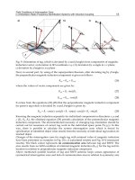
A block diagram of a thermal diffusivity apparatus and a sample holder are presented in Figure 6.26. A
polymer film (approximate thickness 50 µm) is sandwiched between glass plates, the inner surfaces of
which have been sputtered with gold. One sputtered layer is used as a heating plate and the other as a
resistance sensor. Thick strips of gold are sputtered on top of the original sputtered layer so that the
electrical connections can be made. The edges of the glass plates are sealed with an epoxy resin. For
liquid samples a spacer is placed between the plates. The glass assembly is placed on a copper hot-stage
whose temperature is controlled by a temperature programmer. An alternating electric current is applied
using a function synthesizer to the heating plate, and the Joule heat induces a temperature wave which
propagates through the

file:///Q|/t_/t_145.htm2/13/2006 12:59:10 PM
Document
Page 146
Figure 6.26.
(A) Schematic diagram of
a thermal diffusivity apparatus. (B)
Preparation of sample for TD measure-
ment (courtesy of T. Hashimoto)
sample. Temperature fluctuations in the rear surface of the sample are detected as a variation in the

electrical resistance of the gold layer. The phase lag between the signal applied to the heating plate by
the function synthesizer and the voltage measured at the rear surface is measured using a lock-in
amplifier.

file:///Q|/t_/t_146.htm2/13/2006 12:59:17 PM
Document
Page 147
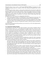
Figure 6.27.
Thermal diffusivity of n-alkane as a function of
temperature and the corresponding DSC curve. The low-
temperature feature is due to a crystal-to-crystal transition
and the high-temperature feature to melting
The periodic temperature fluctuation can be described using the thermal diffusion equation assuming
one-dimensional heat diffusion in the sample, good thermal contact between the sample and glass plate
via the sputtered gold layer and that the temperature of the glass remains constant. Under these
assumptions, the phase lag ∆
θ
is given by
where α is the thermal diffusivity and d the sample thickness.
The thermal diffusivity of an n-alkane as a function of temperature and the corresponding DSC curve
are presented in Figure 6.27. The peak on the low-temperature side of the DSC curve is attributed to a
crystal-to-crystal transition and on the high-temperature side to melting. The value of α decreases at
each transition temperature.
The following items should be included when presenting the results of a TD measurement:
• type of TD apparatus;
• method of sample preparation including dimensions;
• temperature range and heating rate;
• frequency of applied Joule heat.

file:///Q|/t_/t_147.htm2/13/2006 12:59:18 PM

Document
Page 148
6.9 Thermally Stimulated Current (TSC)
Thermally stimulated current (TSC) spectroscopy is used to characterize the relaxation processes and
structural transitions occurring in samples that have been polarized at a temperature greater than the
temperature where molecular motion in the sample is enhanced and subsequently quenched so that the
high mobility state is frozen. On heating the sample at a controlled rate, depolarization of the polymer
electrets (molecular or ionic dipoles, trapped electrons, mobile ions) occurs and the oriented dipoles,
frozen in the quenched sample, relax to a state of thermal equilibrium. This relaxation process is
observed as a depolarization current, which is typically of the order of picoamperes, and is referred to as
the thermally stimulated current.
A TSC apparatus is schematically illustrated in Figure 6.28. The sample is mounted between parallel
condenser-type electrodes and heated to the depolarization temperature, T
p
, under a controlled
atmosphere. A DC voltage of up to 500 V is applied across the electrodes for a time t
p
, producing an
electric field which polarizes the sample. The sample is then quenched at a constant cooling rate to T
0
,
while maintaining the applied electric field. After quenching, the electric field is extinguished and the
sample heated at a constant rate. A TSC curve (or spectrum) plots the thermally stimulated current
versus temperature. This procedure is illustrated in Figure 6.29(I).
Assuming a Debye-type relaxation process, where all dipoles have a single relaxation time and there are
no interactions between dipoles, the instantaneous thermally stimulated current, (J(t)) is given by
where P(t) denotes the polarization decay and α(t) the relaxation frequency [α(t) = 1/
τ
]. Heating at a
constant rate (ß), the temperature-dependent relaxation time is described by the Arrhenius relation:

Figure 6.28.
Schematic diagram of a thermally stimulated
current apparatus (courtesy of H. Shimizu)

file:///Q|/t_/t_148.htm2/13/2006 12:59:19 PM
Document
Page 149
Figure 6.29.
Poling and heating profiles used to
measure thermally stimulated current. (I) Standard
measurement, (II) partial heating method or peak
cleaning method; (III) thermal sampling method
where τ
0
, ∆H and k denote the pre-exponential factor, activation enthalpy and Boltzmann constant,
respectively. The relaxation time is estimated from the TSC spectrum using (see Figure 6.30)
An Arrhenius plot of log τ(T) versus 1/T yields τ
0i
and ∆H
i
.
Figure 6.30.
Schematic illustration
of a TSC spectrum

file:///Q|/t_/t_149.htm2/13/2006 12:59:20 PM
Document
Page 150
However, in polymer systems there can be many internal relaxation modes and it is unreasonable to
assume that a single relaxation process is responsible for the complex TSC curves typically recorded. In

order to deconvolute complex TSC spectra into individual relaxation processes, where the Debye and
Arrhenius relations are more applicable, two approaches are used. The first approach is called the
partial heating method or peak cleaning method (Figure 6.29(II)). Following quenching and extinction
of the applied electric field, the TSC curve of the polarized sample is measured as the sample is heated
at a controlled rate to T
1
. The sample is requenched from T
1
to T
0
, and the TSC curve is subsequently
measured while heating the sample to T
1

+ ∆T at the same rate as before. Typically ∆T≈10 K. The
sample is once again quenched and while heating to T
1
+ 2∆T the TSC curve is again recorded. This
procedure is repeated until the TSC is no longer observed.
The second method is referred to as thermal sampling or thermal windowing [2.3] (Figure 6.29(III)).
The sample is polarized at T
p
for t
p
, which is selected in order to allow orientation of only a portion of
the dipoles present. The sample is quenched to T
p
- ∆T (∆T = 5-10 K) and the electric field removed.
Relaxation occurs at T
p

- ∆T for a time t
d
, which allows partial depolarization of the dipoles to occur.
Finally, the sample is quenched to T
0
. Upon heating at a constant rate a TSC curve is recorded for those
dipoles which did not relax while the sample was maintained at T
p
- ∆T. At T
p
the sample is again
polarized before quenching to T
p
- 2∆T from where the measuring cycle is repeated.
The application of TSC to a wide variety of systems including polymers has been comprehensively
reviewed [4]. Interestingly, the Arrhenius plots (or relaxation maps) of TSC relaxation modes measured
for polymer systems frequently converge to a single point called the compensation point. The physical
meaning of the compensation point is subject to controversy, being possibly the result of the
accumulation of experimental errors. However, it has been claimed that the compensation point defines
two characteristic parameters: the compensation temperature and the compensation time. At the
compensation temperature all modes are proposed to have the same relaxation time, and the degree of
coordination between relaxation modes is an indicator of the thermokinetic state of the amorphous
phase [5].
A wide variety of electrodes are available for measuring samples of different geometrical and physical
forms, including films, fibres, coatings, powders, bulk samples and even liquids (Figure 6.31).
Note that thermally stimulated current spectroscopy cannot be applied to conductive materials with a
resistance smaller than 10
9
Ω/m thickness. In addition, the presence of space charges in the sample can
produce artefacts. For solid samples the upper temperature limit of measurement is the onset of flow,

which presents itself as a large current discharge. This discharge is due to the sample behaving like a
battery and draining the charges accumulated at the surfaces.

file:///Q|/t_/t_150.htm2/13/2006 12:59:21 PM
Document
Page 151
Figure 6.31.
Selection of TSC electrodes. E
indicates the electrode and S the sample
(courtesy of Thermold Partners, LP)
The following items should be included when presenting the results of a TSC measurement:
• type of TSC apparatus;
• method of sample preparation including dimensions;
• type and configuration of electrodes;
• electric field, polarizing temperature and polarizing time;
• quenching rate;
• heating rate and final temperature;
• deconvolution method and associated parameters.
A variation on TSC is thermally stimulated polarization current (TSPC) spectroscopy. In the case of
TSPC the sample is mounted as in TSC. However, the sample is immediately quenched to T
0
without
applying a polarizing electric field. The electric field is then applied and the sample heated at a
controlled rate. The observed current is generated by dipole motion in response to the applied electric
stress. TSPC is a controlled stress technique, unlike TSC which is a relaxation technique. TSPC is
generally used for reactive systems where the heating programme induces a change in the nature of the
sample.
Spontaneous depolarization spectroscopy is like TSPC except that no electric field is applied
whatsoever during the entire course of the experiment. The electrometer measures any current
generated in the sample as a result of dipolar motion over the temperature range of the experiment. This

method can be used, for example, to study the internal stress frozen into a sample during processing.

file:///Q|/t_/t_151.htm2/13/2006 12:59:22 PM
Document
Page 152
6.10 Thermal Conductivity
Quantitative DTAs have been modified by experienced researchers in order to measure the thermal
conductivity of polymer systems [6-8]. The procedure outlined below is reserved for experienced DSC
users. The sample is placed in direct contact with the sample holder, so that the instrument can record
the temperature and the heat flow on one side of the sample. A heat sink of known temperature is
placed in contact with the other side of the sample. Knowing the sample dimensions, the temperature
difference between the sample holder and the heat sink and the recorded heat flow, the thermal
conductivity of the sample can be calculated as follows:
where Q (J) denotes the heat received, t (s) time, κ (W/Km) the sample thermal conductivity, T (K)
temperature, x (m) the sample thickness and A (m
2
) the sample cross-sectional area.
Thermal conductivity measurements by TMDSC [9] involve two experiments on the same sample
material, where only the sample thickness varies. Preparing a sample of uniform and known geometry is
essential for accurate thermal conductivity measurements by this method. The sample is again in direct
contact with the sample holder, so this method is also reserved for experienced users. Selecting a thin
sample, the experimental conditions are chosen so that the heat capacity of the sample can be measured
by the methods outlined earlier (Section 5.6). The second experiment is performed on a thick sample in
such a way that controlled temperature modulation occurs only in that part of the sample in contact with
the sample holder. The remainder of the thick sample functions as a heat sink.
Typical conditions for thermal conductivity measurements by TMDSC [9] are as follows:
• sample mass 10-15 mg (thin sample) and 100-150 mg (thick sample);
• sample dimensions: thickness 3.4-3.8 mm, diameter 6.3 mm;
• constant heating rate 0 K/min, allowing 10-15 min for equilibration before recording data;
• modulated temperature amplitude ±0.5 K;

• modulation period 80 s;
• helium purge 25 ml/min;
• 1 s/data point.
The observed thermal conductivity (κ
ref
) is calculated using

file:///Q|/t_/t_152.htm2/13/2006 12:59:23 PM
Document
Page 153
where x (mm), d (mm) and m (g) are the sample thickness, diameter and mass, respectively, C(J/Kg)
and C
p
(J/K) denote the sample specific heat capacity and apparent heat capacity, respectively, and can
be measured using the methods previously described and p (s) denotes the modulation period.
Measured under the conditions described above [9], the thermal conductivity of the sample (κ) is given
by
where D is the thermal conductivity of the calibration reference material. Using polystyrene as a
standard reference material, D is 0.14 W/Km.
6.11 Micro-thermal Analysis (µTA)
Micro-thermal analysis (µTA
TM
) [10] is a recently developed technique in which the cantilever tip of an
atomic force microscope (AFM) is replaced by a miniature resistive heater. The miniature device is
composed of a small resistance thermometer made from Wollaston wire, enabling the device to function
simultaneously as a resistance heater and a thermal sensor [11]. The modified tip is maintained at a
constant average temperature and a temperature modulation applied. The temperature modulation
frequency is generally in the kHz range. Operating in AFM contact mode, the tip rasters the surface of
the sample, measuring the topography and collecting thermal data. The average DC signal recorded by
the tip depends on the sample thermal conductivity, whereas the response to the AC temperature

modulation is a function of the thermal diffusivity of the near-surface.
The sample surface can be imaged using the topography, thermal conductivity or thermal diffusivity
data. Interesting surface features can be selected from the corresponding image and the tip placed at that
point. The tip temperature is then modulated and the sample response at that point studied, much as in a
conventional DSC experiment it is claimed [10]. However, the volume of the sample being analyzed is
dependent upon the modulation frequency that is chosen so that the AC signal responds to thermal
events close to the tip. The volume sampled by the tip is of the order of a few µm
3
, with a spatial
resolution of about 1 µm. The depth probed by the AC signal is controlled by the modulation frequency.
The transition temperatures measured by µTA tend to differ from bulk measurements. This is due to
surface effects, but there is probably also a contribution from the heating/cooling experiments which are
performed, albeit on tiny sample volumes, at rates exceeding 500 K/min. For the moment calorimetric
data are non-quantitative.
The tip can be used to exert a controlled force at a point on the surface. If temperature modulation is
then applied to the tip the sample may soften or melt

file:///Q|/t_/t_153.htm2/13/2006 12:59:30 PM
Document
Page 154
in the presence of the applied force. It is claimed that this is analogous to a conventional TMA
measurement, and that the extension of this approach, which uses temperature and force modulation, is
analogous to a conventional DMA experiment.
Micro-thermal analysis (µTA
TM
), micro-modulated differential thermal analysis (µMDTA
TM
) and
micro-thermomechanical analysis (µTMA
TM

) are registered trade marks of TA Instruments Inc. For the
time being little work has been reported using such instruments [12] and the calorimetric data are non-
quantitative, so that results from µTA should be interpreted with caution.
6.12 Optothermal Transient Emission Radiometry (OTTER)
In optothermal transient emission radiometry a sample material is irradiated (excited) with optical
wavelength radiation in the form of short-duration pulses and the thermal emission transient observed
by means of a wide-band infrared detector (Figure 6.32). An optothermal decay curve plots the intensity
of the thermal emission versus time. The shape of the decay curve depends upon the extent to which the
incident radiation penetrates into the sample, as well as on the thermal diffusivity and transparency to
the emitted thermal infrared of the material.
Considering that the thermal emission, S(t), emanates only from the surface of the sample and that the
overall temperature increase is small compared to the sample temperature, the following relation can be
derived:
where T denotes the absolute temperature of the sample, ε and σ are the surface emissivity and Stefan's
constant, respectively. θ
0
is the initial temperature rise at
Figure 6.32.
Schematic illustration of an
optothermal transient emission
radiometry (OTTER) apparatus

file:///Q|/t_/t_154.htm2/13/2006 12:59:31 PM
Document
Page 155
the sample surface, erfc the complementary error function and A = α
2
δ, where α is the absorption
coefficient for the incident radiation and δ the sample thermal diffusivity. The thermal characteristics of
the sample are estimated by adjusting the values of the parameters of equation 6.26 to fit the

experimental optothermal decay curve.
The incident radiation is provided by a laser pulse (wavelength 360-760 nm, duration 1-15 ns, pulse rate
1-100 Hz, energy 15-30 µJ). The illuminated area is typically 0.5 mm in diameter and the final
temperature decay curve is accumulated following up to 10 000 laser pulses. This technique is suitable
for the in situ non-destructive study of surfaces, and has been used to measure the thermal diffusivity of
polyester films [13] and pigments [14]. More recently OTTER has been extended to the in vivo study of
water concentration gradients in the stratum corneum [15]. The principle drawback of OTTER is that
the values of the estimated parameters are entirely model dependent and improving the quality of
experimental models is the major focus of current research in this field.
6.13 Specific Heat Spectroscopy
Specific heat spectroscopy (SHS) is a non-adiabatic technique used to measure the frequency-dependent
heat capacity of organic materials near the glass transition over a wide frequency range [16]. Using the
fact that molecular relaxation times increase rapidly as the glass transition is approached from T > T
g
,
the dynamics of the liquid phase (and not the glassy phase) can be studied. In practice a sinusoidally
varying current of frequency ω/2 is supplied by a resistance element which is immersed in the liquid
sample. The resistance element functions both as a heater and as a thermocouple, and its shape is
variable with both linear and planar forms used. The alternating current produces a modulation of the
heater temperature (T
ω
). The power dissipated has two components: a DC component which produces a
constant temperature gradient in the sample and an AC component which produces diffusive thermal
waves. The electrical resistance of the heater varies with T
ω
and is therefore also modulated. The
voltage loss across the heater at a specific frequency (3ω/2) is proportional to T
ω
, from which C
p

κ can
be estimated using the following relation:
assuming that the heater has a planar geometry of infinite area and zero thickness. A is a constant which
depends on the heater current and C
p
and κ denote the sample heat capacity and thermal conductivity,
respectively. The subscript ref indicates measurements made using an empty sample holder over the
entire temperature range of the experiment. Note that SHS measures the product C
p
κ and not the
individual values.

file:///Q|/t_/t_155.htm2/13/2006 12:59:32 PM
Document
Page 156
Figure 6.33.
Real and imaginary parts of C
p
κ for propylene
glycol as a function of temperature at various frequencies:
_._._, 0.11; 4; - - - -, 110; and ——, 1900
Hz. (Reproduced by permission from N.O. Birge,
Physical Review B, 34, 1631, 1986. ( 1986
by the American Physical Society)
Figure 6.33 presents the real and imaginary components of C
p
κ for propylene glycol as a function of
temperature at various frequencies [17]. The real component is visually similar to the corresponding
DSC data (Sections 5.4 and 5.5). However, the data of Figure 6.33 are reversible, so that no difference
is observed between data recorded on the heating and the cooling cycles. SHS measurements are made

under equilibrium conditions in the regime where the sample responds linearly to small perturbations
from equilibrium.
Typically the sample is maintained at a fixed temperature for 1 h and C
p
κ is measured over the entire
available frequency range (0.035-3.5 kHz) [16]. The temperature is then lowered by 1 K over a 15 min
period and the measuring cycle is repeated. The amplitude of T
ω
varies between 0.001 and 0.1 K.
It has been suggested that at the lower frequencies C
p
κ
includes contributions from all degrees of
freedom in the liquid sample, whereas at higher frequencies only the fast relaxation modes contribute.
In addition, it has been shown, by varying the heater geometry, that the frequency dependence of C
p
κ is
primarily due to the frequency dependence of C
p
[17].
6.14 References
[1] Hatta, I. , Takahashi, H. , Matuoka, S. and Amemiya, Y. Thermochimica Acta 253, 149 (1995).
[2] Lacabanne, C. PhD Thesis, University of Toulouse, France (1974).
[3] Chatain, D. PhD Thesis, University of Toulouse, France (1974).

file:///Q|/t_/t_156.htm2/13/2006 12:59:33 PM