Volume 17 - Nondestructive Evaluation and Quality Control Part 5 doc
Bạn đang xem bản rút gọn của tài liệu. Xem và tải ngay bản đầy đủ của tài liệu tại đây (2.29 MB, 80 trang )
Fig. 27 Variations of the magabsorption signal and stress with strain for an annealed nickel plated 3 mm (
in.) diam aluminum rod
These meager data show that with a calibration curve, the stress in nonferromagnetic materials can be measured using the
magabsorption signals from a thin nickel plating on the nonferromagnetic material. The magabsorption versus stress
graph for the nickel plated aluminum seems to obey nearly the same equation as does the nickel wire. To date, no
measurements of the stress in bars of aluminum with small areas of nickel plating have been accomplished as yet, but are
planned for the future.
Residual Stresses and Magnetism. Asymmetries in magabsorption signals may be indicative of residual stresses or
magnetism. In the case of residual magnetism, the magnetic domains are not entirely haphazard; instead they do some
ordering in a particular direction (Fig. 4f). This will produce asymmetries in the magnitude of the magabsorption signal,
depending on the orientation of the bias field, H
B
, with respect to the orientation of the residual magnetism.
Similarly, residual stresses are indicated by the ratio of magabsorption signals from two orientations (0°, 90°) of the bias
coil. When the 0° and 90° amplitudes are equal, the stress is zero whatever the amplitudes are. When the
parallel/perpendicular ratio is greater than 1, the stress value is positive and is tensile; when the ratio is less than 1, the
stress is negative or compressive. For example, in one investigation, magabsorption measurements were made on steel
samples before and after turning, cutting, and shaping operations. For the turning operation, the sample was reduced in
diameter with a cutting tool; for the cutting operation, a sample was reduced in thickness by a ram shaper; for the shaping
operation, the sample was reduced in thickness by an end mill. With the turning operation, the ratio of the 0° to the 90°
magnitude of the magabsorption decreased from 0.91 to 0.89 when a 130 m (5 mil) cut was made. When a 230 m (9
mil) cut was made, the magabsorption ratio decreased from 0.89 to 0.65. When a 500 m (20 mil) cut was made, the
magabsorption ratio decreased from 0.65 to 0.60. These changes indicated that the turning operation was placing
compressive stress on the testpiece. The testpiece used with the ram shaper was in tension along its length before being
reduced in width. A reduction in width of 760 m (30 mils) by the ram shaper applied perpendicular to the length caused
the surface magabsorption signal ratio to indicate compression after the reduction. With the end mill, the reduction in
thickness resulted in the stress changing from tensile to compressive.
Example 1: Magabsorption Measurement of Residual Stress in a Crankshaft Throw.
Quantitative estimates of residual stress from magabsorption measurements were also performed on a large crank-shaft
throw (Fig. 28) made of 5046 steel. The estimates first required the development of calibration curves as described below.
Fig. 28
Magabsorption detector and three detector heads used to perform measurements on the throw of the
crankshaft shown on the left. A closeup view of the detector heads is shown in Fig. 20.
The calibration curves were developed from two samples made of the same material as the crankshaft throw (type 5046
steel). The graph of the parallel-versus-perpendicular peak-to-peak values of the magabsorption signals from two of the
calibration samples are given in Fig. 29. Two straight lines at angles of 45 and 50° relative to the horizontal axis are also
drawn in Fig. 29. The one at 45° is a zero-stress line where the parallel and perpendicular magabsorption signals are the
same magnitude. The line at 50° is the calibration line to be used to determine the calibration constant for the estimate of
residual stress from the magabsorption measurements. Five stress levels (A, B, C, D, and E in Fig. 29) were applied at the
measuring point on each test bar, and the calibration constant was determined as described below.
Fig. 29 Graph showing the
plot of the parallel/perpendicular ratios for sample 6 (type 5046 steel) and sample 7
(type 5046 steel)
Previous experiments have indicated that the intersections of the parallel and perpendicular magnitudes for magabsorption
signals at one point for the residual stresses seldom occur along the same line as applied stresses. However, it has been
indicated that the applied stress lines in Fig. 29 probably can be used to determine the residual stress values in general by
following the rule: All points on a radial line from the origin at some angle with respect to the abscissa have the same
value of residual stress. The 45° line should be the locus of points of zero stress where the parallel and perpendicular
values of the magabsorption curve are equal. With the 45° line as a reference, residual or applied stress can be expressed
mathematically as:
(Eq 19)
where K is the calibration constant for the material. When the parallel and perpendicular amplitudes are equal, the stress
is zero whatever the amplitudes are. When the parallel/perpendicular ratio is greater than one, the stress value is positive
and is tension; when the ratio is less than one, the stress is negative or compression.
The calibration constant, K, is obtained from Fig. 29 by the following procedure: (a) draw a calibration line through the
origin at an angle for which an applied stress can be assigned to the intersection of the parallel/perpendicular ratio for the
applied stress and (b), calculate the value of the constant K by inserting the applied stress and the angle into Eq 19.
Before this procedure could be used with the data in Fig. 29, the usable applied stress curve had to be chosen. One of the
applied stress curves from sample No. 7 was chosen because its amplitude was the closest to the residual stress data, and
because its curve shape was close to that obtained from the throw. The calibration proceeded as described. The line at 50°
was chosen for the first calibration value because it intersected the lowest amplitude (dashed curve) for the data from
sample 7 at nearly the value of applied stress level B (closed circle) (55 MPa, or 8 ksi). The 45° line passes through the
No. 7 stress curve (dashed) nearly at level C (open triangle), or where an estimated value of 160 MPa (23.5 ksi) had been
applied. Therefore, the line at an angle of 50° represents a differential applied stress relative to the 45° line of 160 - 55 =
105 MPa (23.5 - 8 = 15.5 ksi). When several values are taken from several lines both above and below the 45° line, the
average value for a line 5° above or below 45° is 100 MPa (15 ksi). Therefore, if both the value of tan
-1
50° and the stress
equal to 100 MPa (15 ksi) are inserted into Eq 19, the value of K is found to be 20 MPa/degree (3 ksi/degree). This
implies that for every degree of offset from the 45° line, points along the line at that offset resulting from signal amplitude
measurements will have the same value of residual stress.
When the value of K is used, calibration lines can be drawn through zero at useful angles relative to the 45° line. Using
these calibration lines and marks, the values of the residual stresses for points on the crankshaft throw were determined.
Residual stress values as high as 600 MPa (87 ksi) tension and 90 MPa (13 ksi) compression were determined.
References cited in this section
3. W.L. Rollwitz, "Magnetoabsorption," Final Report, Research Project No. 712-
4, Southwest Research
Institute, 1958
4. W.L. Rollwitz and A.W. Whitney, "Special Te
chniques for Measuring Material Properties," Technical
Report ASD-TDR-64-123, USAF Contract No. AF-33(657)-10326, Air Force Materials Laboratory, 1964
5.
W.L. Rollwitz and J.P. Classen, "Magnetoabsorption Techniques for Measuring Material Properties,"
Technical Report AFML-TR-65-17, USAF Contract No. AF-33(657)-
10326, Air Force Materials
Laboratory, 1965
6.
W.L. Rollwitz and J.P. Classen, "Magnetoabsorption Techniques for Measuring Material Properties,"
Technical Report AFML-TR-66-76 (Part I), USAF Contract No. AF-33(657)-
10326, Air Force Materials
Laboratory, 1966
7.
W.L. Rollwitz, "Magnetoabsorption Techniques for Measuring Material Properties. Part II. Measurements
of Residual and Applied Stress." Technical Report AFML-TR-66-76 (Part II), USAF Contract No. AF-
33(615)-5068, Air Force Materials Laboratory, 1968
11.
W.L. Rollwitz, "Preliminary Magnetoabsorption Measurements of Stress in a Crankshaft Throw," Summary
Report on Project 15-2438, Southwest Research Institute, 1970
Magabsorption NDE
William L. Rollwitz, Southwest Research Institute
References
1. W.E. Bell, Magnetoabsorption,
Vol 2, Proceedings of the Conference on Magnetism and Magnetic
Materials, American Institute of Physics, 1956, p 305
2. R.M. Bozorth, Magnetism and Electrical Properties, in Ferromagnetism, D. Van Nostrand, 1951, p 745-
768
3. W.L. Rollwitz, "Magnetoabsorption," Final Report, Research Project No. 712-
4, Southwest Research
Institute, 1958
4. W.L. Rollwitz and A.W. Whitney, "Special Techniques for Measuring Material Properti
es," Technical
Report ASD-TDR-64-123, USAF Contract No. AF-33(657)-10326, Air Force Materials Laboratory, 1964
5.
W.L. Rollwitz and J.P. Classen, "Magnetoabsorption Techniques for Measuring Material Properties,"
Technical Report AFML-TR-65-17, USAF Contract No. AF-33(657)-
10326, Air Force Materials
Laboratory, 1965
6.
W.L. Rollwitz and J.P. Classen, "Magnetoabsorption Techniques for Measuring Material Properties,"
Technical Report AFML-TR-66-76 (Part I), USAF Contract No. AF-33(657)-10326, Air Force Mater
ials
Laboratory, 1966
7.
W.L. Rollwitz, "Magnetoabsorption Techniques for Measuring Material Properties. Part II. Measurements
of Residual and Applied Stress." Technical Report AFML-TR-66-76 (Part II), USAF Contract No. AF-
33(615)-5068, Air Force Materials Laboratory, 1968
8. W.L. Rollwitz, Magnetoabsorption, Progress in Applied Materials Research,
Vol 6, E.G. Stanford, J.H.
Fearon, and W.J. McGonnagle, Ed., Heywood, 1964
9. W.L. Rollwitz, Sensing Apparatus for Use With Magnetoabsorption Apparatus, U.S.
Patent 3,612,968,
1971
10.
W.L. Rollwitz, J. Arambula, and J. Classen, Method of Determining Stress in Ferromagnetic Members
Using Magnetoabsorption, 1974
11.
W.L. Rollwitz, "Preliminary Magnetoabsorption Measurements of Stress in a Crankshaft Throw,"
Summary Report on Project 15-2438, Southwest Research Institute, 1970
Electromagnetic Techniques for Residual Stress Measurements
H. Kwun and G.L. Burkhardt, Southwest Research Institute
Introduction
RESIDUAL STRESSES in materials can be nondestructively measured by a variety of methods, including x-ray
diffraction, ultrasonics, and electromagnetics (Ref 1, 2, 3). With the x-ray diffraction technique, the interatomic planar
distance is measured, and the corresponding stress is calculated (Ref 4). The penetration depth of x-rays is of the order of
only 10 in. (400 in.) in metals. Therefore, the technique is limited to measurements of surface stresses. Its use has been
generally limited to the laboratory because of the lack of field-usable equipment and concern with radiation safety.
With ultrasonic techniques, the velocity of the ultrasonic waves in materials is measured and related to stress (Ref 5).
These techniques rely on a small velocity change caused by the presence of stress, which is known as the acoustoelastic
effect (Ref 6). In principle, ultrasonic techniques can be used to measure bulk as well as surface stresses. Because of the
difficulty in differentiating stress effects from the effect of material texture, practical ultrasonic applications have not yet
materialized.
With electromagnetic techniques, one or more of the magnetic properties of a material (such as permeability,
magnetostriction, hysteresis, coercive force, or magnetic domain wall motion during magnetization) are sensed and
correlated to stress. These techniques rely on the change in magnetic properties of the material caused by stress; this is
known as the magnetoelastic effect (Ref 7). These techniques, therefore, apply only to ferromagnetic materials, such as
steel.
Of the many electromagnetic stress-measurement techniques, this article deals with three specific ones: Barkhausen noise,
non-linear harmonics, and magnetically induced velocity changes. The principles, instrumentation, stress dependence, and
capabilities and limitations of these three techniques are described in the following sections.
References
1.
M.R. James and O. Buck, Quantitative Nondestructive Measurements of Residual Stresses, CRC Crit.
Rev.
Solid State Mater. Sci., Vol 9, 1980, p 61
2.
C.O. Ruud, "Review and Evaluation of Nondestructive Methods for Residual Stress Measurement," Final
Report, NP-1971, Project 1395-5, Electric Power Research Institute, Sept 1981
3.
W.B. Young, Ed., Residual Stress in Design, Process, and Material Selection,
Proceedings of the ASM
Conference on Residual Stress in Design, Process, and Materials Selection, Cincinnati, OH,
April 1987,
ASM INTERNATIONAL, 1987
4.
M.R. James and J.B. Cohen, The Measurement of Residual Stresses by X-
Ray Diffraction Techniques, in
Treatise on Materials Science and Technology Experimental Methods,
Vol 19A, H. Herman, Ed., Academic
Press, 1980, p 1
5.
Y. H. Pao, W. Sachse, and H. Fukuoka, Acoustoelasticity and Ultrasonic Measurement of Residual Stresses,
in Physical Acoustics: Principles and Methods,
Vol XVII, W.P. Mason and R.M. Thurston, Ed., Academic
Press, 1984, p 61-143
6.
D.S. Hughes and J.L. Kelly, Second-Order Elastic Deformation of Solids, Phys. Rev., Vol 92, 1953, p 1145
7.
R.M. Bozorth, Ferromagnetism, Van Nostrand, 1951
Electromagnetic Techniques for Residual Stress Measurements
H. Kwun and G.L. Burkhardt, Southwest Research Institute
Barkhausen Noise
The magnetic flux density in a ferromagnetic material subjected to a time-varying magnetic field does not change in a
strictly continuous way, but rather by small, abrupt, discontinuous increments called Barkhausen jumps (after the name of
the researcher who first observed this phenomenon), as illustrated in Fig. 1. The jumps are due primarily to discontinuous
movements of boundaries between small magnetically saturated regions called magnetic domains in the material (Ref 7,
8, 9). An unmagnetized macroscopic specimen consists of a great number of domains with random magnetic direction so
that the average bulk magnetization is zero. Under an external magnetic field, the specimen becomes magnetized mainly
by the growth of volume of domains oriented close to the direction of the applied field, at the expense of domains
unfavorably oriented. The principal mechanism of growth is the movement of the walls between adjacent domains.
Because of the magnetoelastic interaction, the direction and magnitude of the mechanical stress strongly influence the
distribution of domains and the dynamics of the domain wall motion and therefore the behavior of Barkhausen jumps
(Ref 8). This influence, in turn, is used for stress measurements. Because the signal produced by Barkhausen jumps
resembles noise, the term Barkhausen noise is often used.
Fig. 1 Hysteresis loop for magnetic material showing discontinuities that produce Barkhausen noise.
Source:
Ref 2
Instrumentation. The arrangement illustrated in Fig. 2 is used for the Barkhausen noise technique (Ref 8). A small C-
shaped electromagnet is used to apply a controlled, time-varying magnetic field to the specimen. The abrupt movements
of the magnetic domains are typically detected with an inductive coil placed on the specimen. The detected signal is a
burst of noiselike pulses, as illustrated in Fig. 3. Certain features of the signal, such as the maximum amplitude or root
mean square (rms) amplitude of the Barkhausen noise burst or the applied magnetic field strength at which the maximum
amplitude occurs, are used to determine the stress state in the material (Ref 1, 8, 9, 10, 11, and 12).
Fig. 2 Arrangement for sensing the Barkhausen effect
Fig. 3 Schematic showing the change in magnetic field H
with time, variation in flux density over the same
period, and the generation of the Barkhausen noise burst as flux density changes. Source: Ref 14
In addition to inductive sensing of the magnetic Barkhausen noise, magnetoacoustic Barkhausen activity can also be
detected with an acoustic emission sensor (Ref 13). This phenomenon occurs when Barkhausen jumps during the
magnetization of a specimen produce mechanical stress pulses in a manner similar to the inductive Barkhausen noise
burst shown in Fig. 3. It is caused by microscopic changes in strain due to magnetostriction when discontinuous,
irreversible domain wall motion of non-180° domain walls occurs (Ref 14, 15). This acoustic Barkhausen noise is also
dependent on the stress state in the material and can therefore be used for stress measurements (Ref 15, 16, 17, 18, and
19).
Stress Dependence. The magnetic Barkhausen effect is dependent on the stress as well as the relative direction of the
applied magnetic field to the stress direction. To illustrate this, Fig. 4 shows a typical stress dependence of the inductively
detected Barkhausen noise in a ferrous material. In the case where the magnetic field and the stress are parallel, the
Barkhausen amplitude increases with tension and decreases with compression (Ref 8, 10, 20, and 21). In the case where
the two are perpendicular, the opposite result is obtained. The behavior shown in Fig. 4 holds for materials with a positive
magnetostriction coefficient; for materials with a negative magnetostriction, the Barkhausen amplitude exhibits the
opposite behavior.
Fig. 4 Typical stress dependenc
e of Barkhausen noise signal amplitude with the applied magnetic field parallel
(curve A) and perpendicular (curve B) to the stress direction
For a given stress, the dependence of the Barkhausen amplitude on the angle between the magnetic field and stress
directions is proportional to the strain produced by the stress (Ref 21). Because the Barkhausen noise is dependent on the
strain, Barkhausen measurements can be used as an alternative to strain gages (Ref 20, 21).
A typical stress dependence of the acoustic Barkhausen noise is illustrated in Fig. 5, in which the magnetic field is applied
parallel to the stress direction. As shown, the amplitude of the acoustic signal decreases with tension. Under compression,
it increases slightly and then decreases with an increasing stress level. The acoustic Barkhausen noise, therefore, cannot
distinguish tension from compression.
Fig. 5 Dependence of acoustic emission during the magnetization of low-
carbon steel on stress. Total gain: 80
dB. Magnetic field strength (rms value): 13,000 A/m (160 Oe) for curve A; 6400 A/m (80 Oe) for curve B.
Source: Ref 13
Capabilities and Limitations. Because of the eddy current screening, the inductively detected Barkhausen noise
signals reflect the activity occurring very near the surface of the specimen to a depth of approximately 0.1 mm (0.004 in.).
Therefore, the Barkhausen noise technique is suitable for measuring near-surface stresses. The effective stress-
measurement range is up to about 50% of the yield stress of the material because the change in the Barkhausen noise with
stress becomes saturated at these high stress levels.
Barkhausen measurements can usually be made within a few seconds. Continuous measurements at a slow scanning speed
( 10 mm/s, or 0.4 in./s) are possible. Preparation of the surface of a part under testing is generally not required. Portable,
field-usable Barkhausen instruments are available.
The results of Barkhausen noise measurements are also sensitive to factors not related to stress, such as microstructure,
heat treatment, and material variations. Careful instrument calibration and data analysis are essential for reliable stress
measurements. As can be seen in Fig. 4, the Barkhausen amplitude at zero stress is approximately isotropic and shows no
dependence on the relative orientation of the magnetic field and stress directions. When the specimen is subjected to a
stress, the Barkhausen noise exhibits dependence on the magnetic field direction and becomes anisotropic. This stress-
induced anisotropy in the Barkhausen noise is effective for differentiating stress from nonstress-related factors whose
effects are approximately isotropic. The accuracy of the technique is about ±35 MPa (±5 ksi).
The acoustic Barkhausen noise technique can be used in principle to measure bulk stresses in materials because the
acoustic waves travel through materials. However, practical application of this technique is currently hampered by the
difficulty in differentiating acoustic Barkhausen noise from other noise produced from surrounding environments.
The inductive Barkhausen noise technique has been used for measuring welding residual stresses (Ref 20, 22), for
detecting grinding damage in bearing races (Ref 23), and for measuring compressive hoop stresses in railroad wheels (Ref
24).
References cited in this section
1. M.R. James and O. Buck, Quantitative Nondestructive Measurements of Residual Stresses, CRC Crit.
Rev.
Solid State Mater. Sci., Vol 9, 1980, p 61
2.
C.O. Ruud, "Review and Evaluation of Nondestructive Methods for Residual Stress Measurement," Final
Report, NP-1971, Project 1395-5, Electric Power Research Institute, Sept 1981
7. R.M. Bozorth, Ferromagnetism, Van Nostrand, 1951
8.
G.A. Matzkanin, R.E. Beissner, and C.M. Teller, "The Barkhausen Effect and Its Applications to
Nondestructive Evaluation," State of the Art Report, NTIAC-79-
2, Nondestructive Testing Information
Analysis Center, Southwest Research Institute, Oct 1979
9. J.C. McClure, Jr., and K. Schroder, The Magnetic Barkhausen Effect, CRC Crit. Rev. Solid State Sci.,
Vol
6, 1976, p 45
10.
R.L. Pasley, Barkhausen Effect An Indication of Stress, Mater. Eval., Vol 28, 1970, p 157
11.
S. Tiitto, On the Influence of Microstructure on Magnetization Transitions in Steel, Acta Polytech. Scand.,
No. 119, 1977
12.
R. Rautioaho, P. Karjalainen, and M. Moilanen, Stress Response of Barkhausen Noise and Coercive Force
in 9Ni Steel, J. Magn. Magn. Mater., Vol 68, 1987, p 321
13.
H. Kusanagi, H. Kimura, and H. Sasaki, Acoustic Emission Characteristics During Magnetization of
Ferromagnetic Materials, J. Appl. Phys., Vol 50, 1979, p 2985
14.
D.C. Jiles, Review of Magnetic Methods for Nondestructive Evaluation, NDT Int., Vol
21 (No. 5), 1988, p
311-319
15.
K. Ono and M. Shibata, Magnetomechanical Acoustic Emission of Iron and Steels, Mater. Eval.,
Vol 38,
1980, p 55
16.
M. Shibata and K. Ono, Magnetomechanical Acoustic Emission
A New Method for Nondestructive Stress
Measurement, NDT Int., Vol 14, 1981, p 227
17.
K. Ono, M. Shibata, and M.M. Kwan, Determination of Residual Stress by Magnetomechanical Acoustic, in
Residual Stress for Designers and Metallurgists, L.J. Van de Walls, Ed., American Society for Metals, 1981
18.
G
.L. Burkhardt, R.E. Beissner, G.A. Matzhanin, and J.D. King, Acoustic Methods for Obtaining
Barkhausen Noise Stress Measurements, Mater. Eval., Vol 40, 1982, p 669
19.
K. Ono, "Magnetomechanical Acoustic Emission A Review," Technical Report TR-86-02, Uni
versity of
California at Los Angeles, Sept 1986
20.
G.L. Burkhardt and H. Kwun, "Residual Stress Measurement Using the Barkhausen Noise Method," Paper
45, presented at the 15th Educational Seminar for Energy Industries, Southwest Research Institute, April
1988
21.
H. Kwun, Investigation of the Dependence of Barkhausen Noise on Stress and the Angle Between the Stress
and Magnetization Directions, J. Magn. Magn. Mater., Vol 49, 1985, p 235
22.
L.P. Karjalainen, M. Moilanen, and R. Rautioaho, Evaluating the
Residual Stresses in Welding From
Barkhausen Noise Measurements, Materialprüfung, Vol 22, 1980, p 196
23.
J.R. Barton and F.M. Kusenberger, "Residual Stresses in Gas Turbine Engine Components From
Barkhausen Noise Analysis," Paper 74-GT-51, presented at
the ASME Gas Turbine Conference, Zurich,
Switzerland, American Society of Mechanical Engineers, 1974
24.
J.R. Barton, W.D. Perry, R.K. Swanson, H.V. Hsu, and S.R. Ditmeyer, Heat-
Discolored Wheels: Safe to
Reuse?, Prog. Railroad., Vol 28 (No. 3), 1985, p 44
Electromagnetic Techniques for Residual Stress Measurements
H. Kwun and G.L. Burkhardt, Southwest Research Institute
Nonlinear Harmonics
Because of the magnetic hysteresis and nonlinear permeability, the magnetic induction, B, of a ferromagnetic material
subjected to a sinusoidal, external magnetic field, H, is not sinusoidal but distorted, as illustrated in Fig. 6. This distorted
waveform of the magnetic induction contains odd harmonic frequencies of the applied magnetic field. Mechanical
stresses greatly influence the magnetic hysteresis and permeability of the material (Ref 7). An example of the stress
effects on the hysteresis loops is shown in Fig. 7. Accordingly, the harmonic content of the magnetic induction is also
sensitive to the stress state in the material. With the nonlinear harmonics technique, these harmonic frequencies are
detected, and their amplitudes are related to the state of stress in the material (Ref 26, 27).
Fig. 6 Distortion of m
agnetic induction caused by hysteresis and nonlinearity in magnetization curve. The curve
for magnetic induction, B, is not a pure sinusoid; it has more rounded peaks.
Fig. 7
Hysteresis loops of an AISI 410 stainless steel specimen having ASTM No. 1 grain size and a hardness of
24 HRC under various levels of uniaxial stress. x-axis: 1600 A/m (20 Oe) per division; y-axis: 0.5 T (
5 kG) per
division. Source: Ref 25
Instrumentation. The nonlinear harmonics technique is implemented with the arrangement shown schematically in
Fig. 8. The magnetic field is applied to a specimen with an excitation coil, and the resulting magnetic induction is
measured with a sensing coil. A sinusoidal current of a given frequency is supplied to the excitation coil with a function
generator (or oscillator) and a power amplifier. The induced voltage in the sensing coil is amplified, and the harmonic
frequency content of the signal is analyzed. The amplitude of the harmonic frequency, typically the third harmonics, is
used to determine the stress.
Fig. 8 Block diagram of nonlinear harmonics instrumentation
Stress Dependence. The harmonic amplitudes are dependent on the stress as well as the relative orientation between
the stress and the applied magnetic field directions. Like the stress dependence of the Barkhausen noise amplitude
illustrated in Fig. 4, the harmonic amplitude for materials with a positive magnetostriction increases with tension when
the direction of the stress and the applied field are parallel (Ref 27). When the directions are perpendicular, the opposite
result is obtained. As with Barkhausen noise, the nonlinear harmonics depend on strain and can be used to determine
stress.
Capabilities and Limitations. The nonlinear harmonics technique can be used to measure near-surface stresses, with
sensing depth approximately equal to the skin depth of the applied magnetic field. Because the skin depth is a function of
the frequency of the applied magnetic field, the depth of sensing can be changed by varying the frequency. Therefore, the
technique can potentially be used to measure stress variations with depth.
The results of nonlinear harmonic measurements are sensitive to factors not related to stress, such as microstructure, heat
treatment, and material variations. The stress-induced anisotropy in the harmonic amplitude has been shown to be
effective for differentiating stress from factors not related to stress (Ref 27). When the stress-induced anisotropy is used
for stress determination, the accuracy of the technique is about ±35 MPa (±5 ksi). The range of stress to which the
technique is effective is up to about 50% of the yield stress of the material, with the response becoming saturated at
higher stress levels. With this technique, it would be feasible to measure stress while scanning a part at a high speed ( 10
m/s, or 30 ft/s); therefore, this technique has potential for rapidly surveying stress states in pipelines or continuously
welded railroad rails (Ref 28).
References cited in this section
7. R.M. Bozorth, Ferromagnetism, Van Nostrand, 1951
25.
H. Kwun and G.L. Burkhardt, Effects of Grain
Size, Hardness, and Stress on the Magnetic Hysteresis Loops
of Ferromagnetic Steels, J. Appl. Phys., Vol 61, 1987, p 1576
26.
N. Davis, Magnetic Flux Analysis Techniques, in Research Techniques in Nondestructive Testing,
Vol II,
R.S. Sharpe, Ed., Academic Press, 1973, p 121
27.
H. Kwun and G.L. Burkhardt, Nondestructive Measurement of Stress in Ferromagnetic Steels Using
Harmonic Analysis of Induced Voltage, NDT Int., Vol 20, 1987, p 167
28.
G.L. Burkhardt and H. Kwun, Application of the Nonlinear Harmo
nics Method to Continuous Measurement
of Stress in Railroad Rail, in
Proceedings of the 1987 Review of Progress in Quantitative Nondestructive
Evaluation, Vol 713, D.O. Thompson and D.E. Chimenti, Ed., Plenum Press, 1988, p 1413
Electromagnetic Techniques for Residual Stress Measurements
H. Kwun and G.L. Burkhardt, Southwest Research Institute
Magnetically Induced Velocity Changes (MIVC) for Ultrasonic Waves
Because of the magnetoelastic interaction, the elastic moduli of a ferromagnetic material are dependent on the
magnetization of the material. This phenomenon is known as the E effect (Ref 7). Consequently, the velocity of the
ultrasonic waves in the material changes when an external magnetic field is applied to the material. This MIVC for
ultrasonic waves is characteristically dependent on the stress as well as the angle between the stress direction and the
direction of the applied magnetic field (Ref 29, 30, 31, and 32). This characteristic stress dependence of the MIVC is used
for stress determination (Ref 33, 34, 35, and 36).
Instrumentation. Figure 9 shows a block diagram of instrumentation for measuring MIVC. An electromagnet is used
to apply a biasing magnetic field to the specimen. The applied magnetic field is measured with a Hall probe. An
ultrasonic transducer is used to transmit ultrasonic waves and to detect signals reflected from the back surface of the
specimen. For surface waves, separate transmitting and receiving transducers are used. The shift in the arrival time of the
received ultrasonic wave caused by the velocity change due to the applied magnetic field is detected with an ultrasonic
instrument. Because MIVC is a small effect (of the order of only 0.01 to 0.1%), the measurements are typically made
using the interferometer principle, called the phase comparison technique, in the ultrasonic instrumentation (Ref 33).
Fig. 9 Block diagram of instrumentation for measuring MIVC for ultrasonic waves
Stress Dependence. A typical stress dependence of the MIVC is illustrated in Fig. 10. At zero stress, the MIVC at
first generally increases rapidly with the applied magnetic field, H, and then gradually levels off toward a saturation
value. When the material is subjected to stress, the magnitude of the MIVC decreases, and the shape of the MIVC curve
as a function of H changes. Under tension, the shape of the MIVC curve remains similar to that at zero stress, but with
reduced magnitude in proportion to the stress level. Under compression, the MIVC curve exhibits a minimum, which
drastically changes the shape and reduces the magnitude. The magnitude of the minimum and the value of H where the
minimum occurs increase with stress level.
Fig. 10 Schematic showing the change in ultrasonic velocity, V, with magnetic field H
under various stress
levels,
The detailed stress dependence of MIVC, however, varies with the mode of ultrasonic wave used (longitudinal, shear, or
surface) and with the relative orientation between the stress and the magnetic field directions (Ref 29, 30, 31, 32, 33, 34,
and 35). The stress dependence shown in Fig. 10 holds for longitudinal waves in materials with a positive
magnetostriction coefficient (Ref 31, 33). With this technique, the stress state in the material, including the magnitude,
direction, and sign (tensile or compressive) of the stress, is characterized by analyzing the shape and magnitude of the
MIVC curves measured at two or more different magnetic field directions.
Capabilities and Limitations. The MIVC technique can be used to measure bulk and surface stresses by applying
both bulk (shear or longitudinal) and surface ultrasonic waves. A measurement can be made within a few seconds.
Because the magnitude of MIVC depends on material type, reference or calibration curves must be established for that
material type prior to stress measurements. However, this technique is insensitive to variations in the texture and
composition of nominally the same material. The accuracy in stress measurements is about ±35 MPa (±5 ksi). This
technique has been used to measure residual welding stresses (Ref 34) and residual hoop stresses in railroad wheels Ref
36).
A relatively large electromagnet is needed to magnetize the part under investigation and may be cumbersome to handle in
practical applications. Because of difficulty in magnetizing complex-geometry parts, the application of the technique is
limited to simple geometry parts.
References cited in this section
7. R.M. Bozorth, Ferromagnetism, Van Nostrand, 1951
29.
H. Kwun and C.M. Teller, Tensile Stress Dependence of Magnetically Induced Ultrasonic Shear Wave
Velocity Change in Polycrystalline A-36 Steel, Appl. Phys. Lett., Vol 41, 1982, p 144
30.
H. Kwun and C.M. Teller,
Stress Dependence of Magnetically Induced Ultrasonic Shear Wave Velocity
Change in Polycrystalline A-36 Steel, J. Appl. Phys., Vol 54, 1983, p 4856
31.
H. Kwun, Effects of Stress on Magnetically Induced Velocity Changes for Ultrasonic Longitudinal Waves
in Steels, J. Appl. Phys., Vol 57, 1985, p 1555
32.
H. Kwun, Effects of Stress on Magnetically Induced Velocity Changes for Surface Waves in Steels,
J. Appl.
Phys., Vol 58, 1985, p 3921
33.
H. Kwun, Measurement of Stress in Steels Using Magnetically Indu
ced Velocity Changes for Ultrasonic
Waves, in Nondestructive Characterization of Materials II,
J.F. Bussiere, J.P. Monchalin, C.O. Ruud, and
R.E. Green, Jr., Ed., Plenum Press, 1987, p 633
34.
H. Kwun, A Nondestructive Measurement of Residual Bulk Stresse
s in Welded Steel Specimens by Use of
Magnetically Induced Velocity Changes for Ultrasonic Waves, Mater. Eval., Vol 44, 1986, p 1560
35.
M. Namkung and J.S. Heyman, Residual Stress Characterization With an Ultrasonic/Magnetic Technique,
Nondestr. Test. Commun., Vol 1, 1984, p 175
36.
M. Namkung and D. Utrata, Nondestructive Residual Stress Measurements in Railroad Wheels Using the
Low-Field Magnetoacoustic Test Method, in
Proceedings of the 1987 Review of Progress in Quantitative
Nondestructive Evaluation, Vol 7B, D.O. Thompson and D.E. Chimenti, Ed., Plenum Press, 1988, p 1429
Electromagnetic Techniques for Residual Stress Measurements
H. Kwun and G.L. Burkhardt, Southwest Research Institute
References
1. M.R. James and O. Buck, Quantitative Nondestructive Measurements of Residual Stresses, CRC Crit.
Rev.
Solid State Mater. Sci., Vol 9, 1980, p 61
2.
C.O. Ruud, "Review and Evaluation of Nondestructive Methods for Residual Stress Measurement," Final
Report, NP-1971, Project 1395-5, Electric Power Research Institute, Sept 1981
3. W.B. Young, Ed., Residual Stress in Design, Process, and Material Selection,
Proceedings of the ASM
Conference on Residual Stress in Design, Process, and Materials Selection, Cincinnati, OH, April 1987,
ASM INTERNATIONAL, 1987
4. M.R. James and J.B. Cohen, The Measurement of Residual Stresses by X-
Ray Diffraction Techniques, in
Treatise on Materials Science and Technology Experimental Methods,
Vol 19A, H. Herman, Ed.,
Academic Press, 1980, p 1
5. Y. H. Pao, W. Sachse, and H. Fu
kuoka, Acoustoelasticity and Ultrasonic Measurement of Residual
Stresses, in Physical Acoustics: Principles and Methods,
Vol XVII, W.P. Mason and R.M. Thurston, Ed.,
Academic Press, 1984, p 61-143
6. D.S. Hughes and J.L. Kelly, Second-Order Elastic Deformation of Solids, Phys. Rev.,
Vol 92, 1953, p
1145
7. R.M. Bozorth, Ferromagnetism, Van Nostrand, 1951
8.
G.A. Matzkanin, R.E. Beissner, and C.M. Teller, "The Barkhausen Effect and Its Applications to
Nondestructive Evaluation," State of the Art Report, NTIAC-79-
2, Nondestructive Testing Information
Analysis Center, Southwest Research Institute, Oct 1979
9. J.C. McClure, Jr., and K. Schroder, The Magnetic Barkhausen Effect, CRC Crit. Rev. Solid State Sci.,
Vol
6, 1976, p 45
10. R.L. Pasley, Barkhausen Effect An Indication of Stress, Mater. Eval., Vol 28, 1970, p 157
11. S. Tiitto, On the Influence of Microstructure on Magnetization Transitions in Steel, Acta Polytech. Scand.,
No. 119, 1977
12. R. Rautioaho, P. Karjalainen, and M. Moilanen, Stress Respo
nse of Barkhausen Noise and Coercive Force
in 9Ni Steel, J. Magn. Magn. Mater., Vol 68, 1987, p 321
13.
H. Kusanagi, H. Kimura, and H. Sasaki, Acoustic Emission Characteristics During Magnetization of
Ferromagnetic Materials, J. Appl. Phys., Vol 50, 1979, p 2985
14. D.C. Jiles, Review of Magnetic Methods for Nondestructive Evaluation, NDT Int.,
Vol 21 (No. 5), 1988, p
311-319
15. K. Ono and M. Shibata, Magnetomechanical Acoustic Emission of Iron and Steels, Mater. Eval.,
Vol 38,
1980, p 55
16. M. Shibata and K. Ono, Magnetomechanical Acoustic Emission
A New Method for Nondestructive
Stress Measurement, NDT Int., Vol 14, 1981, p 227
17.
K. Ono, M. Shibata, and M.M. Kwan, Determination of Residual Stress by Magnetomechanical Acoustic,
in Residual Stress for Designers and Metallurgists,
L.J. Van de Walls, Ed., American Society for Metals,
1981
18.
G.L. Burkhardt, R.E. Beissner, G.A. Matzhanin, and J.D. King, Acoustic Methods for Obtaining
Barkhausen Noise Stress Measurements, Mater. Eval., Vol 40, 1982, p 669
19. K. Ono, "Magnetomechanical Acoustic Emission A Review," Technical Report TR-86-
02, University of
California at Los Angeles, Sept 1986
20.
G.L. Burkhardt and H. Kwun, "Residual Stress Measurement Using the Barkhausen Noise Method," Paper
45, pre
sented at the 15th Educational Seminar for Energy Industries, Southwest Research Institute, April
1988
21.
H. Kwun, Investigation of the Dependence of Barkhausen Noise on Stress and the Angle Between the
Stress and Magnetization Directions, J. Magn. Magn. Mater., Vol 49, 1985, p 235
22.
L.P. Karjalainen, M. Moilanen, and R. Rautioaho, Evaluating the Residual Stresses in Welding From
Barkhausen Noise Measurements, Materialprüfung, Vol 22, 1980, p 196
23. J.R. Barton and F.M. Kusenberger, "Residual Stresse
s in Gas Turbine Engine Components From
Barkhausen Noise Analysis," Paper 74-GT-
51, presented at the ASME Gas Turbine Conference, Zurich,
Switzerland, American Society of Mechanical Engineers, 1974
24. J.R. Barton, W.D. Perry, R.K. Swanson, H.V. Hsu, and S.R. Ditmeyer, Heat-
Discolored Wheels: Safe to
Reuse?, Prog. Railroad., Vol 28 (No. 3), 1985, p 44
25.
H. Kwun and G.L. Burkhardt, Effects of Grain Size, Hardness, and Stress on the Magnetic Hysteresis
Loops of Ferromagnetic Steels, J. Appl. Phys., Vol 61, 1987, p 1576
26. N. Davis, Magnetic Flux Analysis Techniques, in Research Techniques in Nondestructive Testing,
Vol II,
R.S. Sharpe, Ed., Academic Press, 1973, p 121
27. H. Kwun and G.L. Burkhardt, Nondestructive Measurement of Stress in Ferromagnetic
Steels Using
Harmonic Analysis of Induced Voltage, NDT Int., Vol 20, 1987, p 167
28.
G.L. Burkhardt and H. Kwun, Application of the Nonlinear Harmonics Method to Continuous
Measurement of Stress in Railroad Rail, in Proceedings of the 1987 Review of Progr
ess in Quantitative
Nondestructive Evaluation, Vol 713, D.O. Thompson and D.E. Chimenti, Ed., Plenum Press, 1988, p 1413
29.
H. Kwun and C.M. Teller, Tensile Stress Dependence of Magnetically Induced Ultrasonic Shear Wave
Velocity Change in Polycrystalline A-36 Steel, Appl. Phys. Lett., Vol 41, 1982, p 144
30.
H. Kwun and C.M. Teller, Stress Dependence of Magnetically Induced Ultrasonic Shear Wave Velocity
Change in Polycrystalline A-36 Steel, J. Appl. Phys., Vol 54, 1983, p 4856
31. H. Kwun, Effects of
Stress on Magnetically Induced Velocity Changes for Ultrasonic Longitudinal Waves
in Steels, J. Appl. Phys., Vol 57, 1985, p 1555
32. H. Kwun, Effects of Stress on Magnetically Induced Velocity Changes for Surface Waves in Steels,
J.
Appl. Phys., Vol 58, 1985, p 3921
33.
H. Kwun, Measurement of Stress in Steels Using Magnetically Induced Velocity Changes for Ultrasonic
Waves, in Nondestructive Characterization of Materials II,
J.F. Bussiere, J.P. Monchalin, C.O. Ruud, and
R.E. Green, Jr., Ed., Plenum Press, 1987, p 633
34.
H. Kwun, A Nondestructive Measurement of Residual Bulk Stresses in Welded Steel Specimens by Use of
Magnetically Induced Velocity Changes for Ultrasonic Waves, Mater. Eval., Vol 44, 1986, p 1560
35. M. Namkung and J.S. Heyman, Residual
Stress Characterization With an Ultrasonic/Magnetic Technique,
Nondestr. Test. Commun., Vol 1, 1984, p 175
36.
M. Namkung and D. Utrata, Nondestructive Residual Stress Measurements in Railroad Wheels Using the
Low-Field Magnetoacoustic Test Method, in Pr
oceedings of the 1987 Review of Progress in Quantitative
Nondestructive Evaluation, Vol 7B, D.O. Thompson and D.E. Chimenti, Ed., Plenum Press, 1988, p 1429
Eddy Current Inspection
Revised by the ASM Committee on Eddy Current Inspection
*
Introduction
EDDY CURRENT INSPECTION is based on the principles of electromagnetic induction and is used to identify or
differentiate among a wide variety of physical, structural, and metallurgical conditions in electrically conductive
ferromagnetic and nonferromagnetic metals and metal parts. Eddy current inspection can be used to:
• Measure or identify such conditions and properties as ele
ctrical conductivity, magnetic permeability,
grain size, heat treatment condition, hardness, and physical dimensions
• Detect seams, laps, cracks, voids, and inclusions
• Sort dissimilar metals and detect differences in their composition, microstructure, and other properties
•
Measure the thickness of a nonconductive coating on a conductive metal, or the thickness of a
nonmagnetic metal coating on a magnetic metal
Because eddy currents are created using an electromagnetic induction technique, the inspection method does not require
direct electrical contact with the part being inspected. The eddy current method is adaptable to high-speed inspection and,
because it is nondestructive, can be used to inspect an entire production output if desired. The method is based on indirect
measurement, and the correlation between the instrument readings and the structural characteristics and serviceability of
the parts being inspected must be carefully and repeatedly established.
Note
* V.S. Cecco, Atomic Energy of Canada L
imited, Chalk River Nuclear Laboratories; E.M. Franklin, Argonne
National Laboratory, Argonne-
West; Howard E. Houserman, ZETEC, Inc.; Thomas G. Kincaid, Boston
University; James Pellicer, Staveley NDT Technologies, Inc.; and Donald Hagemaier, Douglas Aircr
aft
Company, McDonnell Douglas Corporation
Eddy Current Inspection
Revised by the ASM Committee on Eddy Current Inspection
*
Advantages and Limitations of Eddy Current Inspection
Eddy current inspection is extremely versatile, which is both an advantage and a disadvantage. The advantage is that the
method can be applied to many inspection problems provided the physical requirements of the material are compatible
with the inspection method. In many applications, however, the sensitivity of the method to the many properties and
characteristics inherent within a material can be a disadvantage; some variables in a material that are not important in
terms of material or part serviceability may cause instrument signals that mask critical variables or are mistakenly
interpreted to be caused by critical variables.
Eddy Current Versus Magnetic Inspection Methods. In eddy current inspection, the eddy currents create their
own electromagnetic field, which can be sensed either through the effects of the field on the primary exciting coil or by
means of an independent sensor. In nonferromagnetic materials, the secondary electromagnetic field is derived
exclusively from eddy currents. However, with ferromagnetic materials, additional magnetic effects occur that are usually
of sufficient magnitude to overshadow the field effects caused by the induced eddy currents. Although undesirable, these
additional magnetic effects result from the magnetic permeability of the material being inspected and can normally be
eliminated by magnetizing the material to saturation in a static (direct current) magnetic field. When the permeability
effect is not eliminated, the inspection method is more correctly categorized as electromagnetic or magnetoinductive
inspection. Methods of inspection that depend mainly on ferromagnetic effects are discussed in the article "Magnetic
Particle Inspection" in this Volume.
Eddy Current Inspection
Revised by the ASM Committee on Eddy Current Inspection
*
Development of the Inspection Process
The development of the eddy current method of inspection has involved the use of several scientific and technological
advances, including the following:
• Electromagnetic induction
• Theory and application of induction coils
• The solution of boundary-
value problems describing the dynamics of the electromagnetic fields within
the vicinity of induction coils, an
d especially the dynamics of the electromagnetic fields, electric current
flow, and skin effect in conductors in the vicinity of such coils
•
Theoretical prediction of the change in impedance of eddy current inspection coils caused by small
flaws
• Improved
instrumentation resulting from the development of vacuum tubes, semiconductors, integrated
circuits, and microprocessors which led to better measurement techniques and response to subtle
changes in the flow of eddy currents in metals
• Metallurgy and metals fabrication
• Improved instrumentation, signal display, and recording
Electromagnetic induction was discovered by Faraday in 1831. He found that when the current in a loop of wire was
caused to vary (as by connecting or disconnecting a battery furnishing the current), an electric current was induced in a
second, adjacent loop. This is the effect used in eddy current inspection to cause the eddy currents to flow in the material
being inspected and it is the effect used to monitor these currents.
In 1864, Maxwell presented his classical dissertation on a dynamic theory of the electromagnetic field, which includes a
set of equations bearing his name that describe all large-scale electromagnetic phenomena. These phenomena include the
generation and flow of eddy currents in conductors and the associated electromagnetic fields. Thus, all the
electromagnetic induction effects that are basic to the eddy current inspection method are described in principle by the
equations devised by Maxwell for particular boundary values for practical applications.
In 1879, Hughes, using an eddy current method, detected differences in electrical conductivity, magnetic permeability,
and temperature in metal. However, use of the eddy current method developed slowly, probably because such an
inspection method was not needed and because further development of the electrical theory was necessary before it could
be used for practical applications.
Calculating the flow of induced current in metals was later developed by the solution of Maxwell's equations for specific
boundary conditions for symmetrical configurations. These mathematical techniques were important in the electric power
generation and transmission industry, in induction heating, and in the eddy current method of inspection.
An eddy current instrument for measuring wall thickness was developed by Kranz in the mid-1920s. An example of early
well-documented work that also serves as an introduction to several facets of the eddy current inspection method is that of
Farrow, who pioneered in the development of eddy current systems for the inspection of welded steel tubing. He began
his work in 1930 and by 1935 had progressed to an inspection system that included a separate primary energizing coil,
differential secondary detector coil, and a dc magnetic-saturating solenoid coil. Inspection frequencies used were 500,
1000, and 4000 Hz. Tubing diameters ranged from 6.4 to 85 mm ( to 3 in.). The inspection system also included a
balancing network, a high-frequency amplifiers, a frequency discriminator-demodulator, a low-frequency pulse amplifier,
and a filter. These are the same basic elements that are used in modern systems for eddy current inspection.
Several artificial imperfections in metals were tried for calibrating tests, but by 1935 the small drilled hole had become
the reference standard for all production testing. The drilled hole was selected for the standard because:
• It was relatively easy to produce
• It was reproducible
• It could be produced in precisely graduated sizes
• It produced a signal on the eddy curren
t tester that was similar to that produced by a natural
imperfection
• It was a short imperfection and resembled hard-to-
detect, short natural weld imperfections. Thus, if the
tester could detect the small drilled hole, it would also detect most of the natural weld imperfections
Vigners, Dinger, and Gunn described eddy current type flaw detectors for nonmagnetic metals in 1942, and in the early
1940s, Förster and Zuschlag developed eddy current inspection instruments. Numerous versions of eddy current
inspection equipment are currently available commercially. Some of this equipment is useful only for exploratory
inspection or for inspecting parts of simple shape. However, specially designed equipment is extensively used in the
inspection of production quantities of metal sheet, rod, pipe, and tubing.
Eddy Current Inspection
Revised by the ASM Committee on Eddy Current Inspection
*
Principles of Operation
The eddy current method of inspection and the induction heating technique that is used for metal heating, induction
hardening, and tempering have several similarities. For example, both are dependent on the principles of electromagnetic
induction for inducing eddy currents within a part placed within or adjacent to one or more induction coils. The heating is
a result of I
2
R losses caused by the flow of eddy currents in the part. Changes in coupling between the induction coils and
the part being inspected and changes in the electrical characteristics of the part cause variations in the loading and tuning
of the generator.
The induction heating system is operated at high power levels to produce the desired heating rate. In contrast, the system
used in eddy current inspection is usually operated at very low power levels to minimize the heating losses and
temperature changes. Also, in the eddy current system, electrical-loading changes caused by variations in the part being
inspected, such as those caused by the presence of flaws or dimensional changes, are monitored by electronic circuits. In
both eddy current inspection and induction heating, the selection of operating frequency is largely governed by skin effect
(see the section "Operating Variables" in this article). This effect causes the eddy currents to be concentrated toward the
surfaces adjacent to the coils carrying currents that induce them. Skin effect becomes more pronounced with increase in
frequency.
The coils used in eddy current inspection differ from those used in induction heating because of the differences in power
level and resolution requirements, which necessitate special inspection coil arrangements to facilitate the monitoring of
the electromagnetic field in the vicinity of the part being inspected.
Functions of a Basic System. The part to be inspected is placed within or adjacent to an electric coil in which an
alternating current is flowing. As shown in Fig. 1, this alternating current, called the exciting current, causes eddy currents
to flow in the part as a result of electromagnetic induction. These currents flow within closed loops in the part, and their
magnitude and timing (or phase) depend on:
• The original or primary field established by the exciting currents
• The electrical properties of the part
• The electromagnetic fields established by currents flowing within the part
Fig. 1
Two common types of inspection coils and the patterns of eddy current flow generated by the exciting
current in the coils. Solenoid-type coil is applied to cylindrical or tubular parts; pancake-
type coil, to a flat
surface.
The electromagnetic field in the region in the part and surrounding the part depends on both the exciting current from the
coil and the eddy currents flowing in the part. The flow of eddy currents in the part depends on:
• The electrical characteristics of the part
• The presence or absence of flaws or other discontinuities in the part
• The total electromagnetic field within the part
The change in flow of eddy currents caused by the presence of a crack in a pipe is shown in Fig. 2. The pipe travels along
the length of the inspection coil as shown in Fig. 2. In section A-A in Fig. 2, no crack is present and the eddy current flow
is symmetrical. In section B-B in Fig. 2, where a crack is present, the eddy current flow is impeded and changed in
direction, causing significant changes in the associated electromagnetic field. From Fig. 2 it is seen that the
electromagnetic field surrounding a part depends partly on the properties and characteristics of the part. Finally, the
condition of the part can be monitored by observing the effect of the resulting field on the electrical characteristics of the
exciting coil, such as its electrical impedance, induced voltage, or induced currents. Alternatively, the effect of the
electromagnetic field can be monitored by observing the induced voltage in one or more other coils placed within the field
near the part being monitored.
Fig. 2 Effect of a crack on the pattern of eddy current flow in a pipe
Each and all of these changes can have an effect on the exciting coil or other coil or coils used for sensing the
electromagnetic field adjacent to a part. The effects most often used to monitor the condition of the part being inspected
are the electrical impedance of the coil or the induced voltage of either the exciting coil or other adjacent coil or coils.
Eddy current systems vary in complexity depending on individual inspection requirements. However, most systems
provide for the following functions:
• Excitation of the inspection coil
• Modulation of the inspection coil output signal by the part being inspected
• Processing of the inspection coil signal prior to amplification
• Amplification of the inspection coil signals
• Detection or demodulation of the inspection coil signal, usually accom
panied by some analysis or
discrimination of signals
•
Display of signals on a meter, an oscilloscope, an oscillograph, or a strip chart recorder; or recording of
signal data on magnetic tape or other recording media
• Handling of the part being inspected an
d support of the inspection coil assembly or the manipulation of
the coil adjacent to the part being inspected
Elements of a typical inspection system are shown schematically in Fig. 3. The particular elements in Fig. 3 are
for a system developed to inspect bar or tubing. The generator supplies excitation current to the inspection coil and a
synchronizing signal to the phase shifter, which provides switching signals for the detector. The loading of the inspection
coil by the part being inspected modulates the electromagnetic field of the coil. This causes changes in the amplitude and
phase of the inspection coil voltage output.
Fig. 3 Principal elements of a typical system for eddy current inspection of bar or tubing. See description in text.
The output of the inspection coil is fed to the amplifier and detected or demodulated by the detector. The demodulated
output signal, after some further filtering and analyzing, is then displayed on an oscilloscope or a chart recorder. The
displayed signals, having been detected or demodulated, vary at a much slower rate, depending on:
• The speed at which the part is fed through an inspection coil
• The speed with which the inspection coil is caused to scan past the part being inspected
Eddy Current Inspection
Revised by the ASM Committee on Eddy Current Inspection
*
Operating Variables
The principal operating variables encountered in eddy current inspection include coil impedance, electrical conductivity,
magnetic permeability, lift-off and fill factors, edge effect, and skin effect. Each of these variables will be discussed in
this section.
Coil Impedance
When direct current is flowing in a coil, the magnetic field reaches a constant level, and the electrical resistance of the
wire is the only limitation to current flow. However, when alternating current is flowing in a coil, two limitations are
imposed:
• The ac resistance of the wire, R
• A quantity known as inductive reactance, X
L
The ac resistance of an isolated or empty coil operating at low frequencies or having a small wire diameter is very nearly
the same as the dc resistance of the wire of the coil. The ratio of ac resistance to dc resistance increases as either the
frequency or the wire diameter increases. In the discussion of eddy current principles, the resistance of the coil wire is
often ignored, because it is nearly constant. It varies mainly with wire temperature and the frequency and spatial
distribution of the magnetic field threading the coil.