Volume 17 - Nondestructive Evaluation and Quality Control Part 6 doc
Bạn đang xem bản rút gọn của tài liệu. Xem và tải ngay bản đầy đủ của tài liệu tại đây (2.09 MB, 80 trang )
Fig. 52
Eddy current inspection of cracks located under installed bushings. (a) Schematic of typical assembly
employing interference-fit bushings in a clevis/lug attachment asse
mbly. (b) Reference standard incorporating
an electrical discharge machined corner notch. (c) Probe coil positioned in bolthole and encircled by bushing.
(d) CRT display of a crack located under a ferromagnetic bushing. Source: Ref 13
A reference standard was made from material of the proper thickness, and the electrical discharge machined corner notch
was made at the edge of the appropriate-size hole. The bushing was then installed in the reference standard, as shown in
Fig. 52(b). The proper-size bolthole probe was selected and inserted into the bushed hole, and the operating frequency
was selected to allow the eddy current to penetrate through the bushing in order to detect the notch (Fig. 52c and d).
After calibration, the bolthole probe was inserted into the appropriate bushed hole in the lug or crevis on the aircraft. The
probe was inserted at increments of about 1.59 mm (0.0625 in.) and rotated 360° through each hole to be inspected. The
bushing, made of a copper alloy, had a thickness of about 1.5 mm (0.060 in.) and a conductivity between 25 and 30%
IACS, which is easily penetrated at a frequency of 1 to 2 kHz.
Example 14: Detection of Fatigue Cracks in Aircraft Splice Joints.
Surface and subsurface fatigue cracks usually occur at areas of high stress concentration, such as splice joints between
aircraft components or subassemblies. High-frequency (100 to 300 kHz) eddy current inspection was performed to detect
surface cracks with shielded small-diameter probes. A reference standard was made from typical materials, and a small
electrical discharge machining notch was placed at the corner of the external surface adjacent to a typical fastener. The
high-frequency probe was scanned around the periphery of the fastener using a circle template for a guide, as illustrated in
Fig. 53(a).
Fig. 53 High-frequency eddy current inspection of surface
and subsurface cracks in aircraft splice joints. (a)
Calibration procedure involves introducing an electrical discharge machining notch in the reference standard to
scan the fastener periphery using a circle template to guide the probe. (b) CRT trace on an
oscilloscope of
typical cracks in both skin and spar cap sections shown in (c). Source: Ref 13
When subsurface cracks are to be detected, low-frequency eddy current techniques are employed. Basically stated, the
thicker the structure to be penetrated, the lower the eddy current operating frequency that is required. However, the
detectable flaw size usually becomes larger as the frequency is lowered.
Example 15: Hidden Subsurface Corrosion in Windowbelt Panels.
There are various areas of the aircraft where subsurface (hidden) corrosion may occur. If such corrosion is detected,
usually during heavy maintenance teardown, a nondestructive testing method can be developed to inspect these areas in
the remainder of the fleet. Following is an example of subsurface corrosion detected by low-frequency (<10 kHz) eddy
current check of the windowbelt panels. Such inspection is applicable at each window on both sides of the aircraft.
Moisture intrudes past the window seal into the inboard side of the windowbelt panel and causes corrosion thinning of the
inner surface (Fig. 54). The eddy current inspection is performed using a phase-sensitive instrument operating at 1 to 2.5
kHz and either a 6.4 or 9.5 mm (0.25 or 0.375 in.) surface probe.
Fig. 54 Location of subsurface corrosion in aircraft windowbelt panels. Source: Ref 13
The edge of the inner surface of the windowbelt (where corrosion occurs) tapers from 4.06 to 2.0 mm (0.160 to 0.080 in.)
over a distance of 19 mm (0.750 in.). A reference standard simulating various degrees of corrosion thinning (or, in reality,
remaining material thickness) is used to calibrate the eddy current instrument (Fig. 55a). The instrument phase is rotated
slightly so that probe lift-off response is in the horizontal direction of the CRT. As the probe is scanned across the steps in
the standard, the eddy current response is in a vertical direction on the CRT. The amplitude of the response increases as
the material thickness decreases (Fig. 55b). As each step in the standard is scanned, the eddy current response may be
offset, as shown in Fig. 55(c).
Fig. 55
Eddy current calibration procedure to detect subsurface corrosion in the aircraft windowbelt panels
illustrated in Fig. 51
. (a) Reference standard used to simulate varying degrees of corrosion thinning from 0.5 to
2.0 mm (0.020 to 0.08 in.) in 0.5 mm (0.020 in.) increments. (b) Plot of CRT display at 2.25-
kHz test
frequency. (c) CRT offset display permits resolution of amplitudes at the various material thicknesses.
Source:
Ref 13
After calibrating the instrument, the inspector scans along the inner edge of the window and monitors the CRT for
thinning responses, which are indicative of internal corrosion. When thinning responses are noted, the inspection marks
the extent of the corrosion and determines the relative remaining thickness. Results are marked on a plastic overlay or
sketch and submitted to the engineering department for disposition. The extent of severe corrosion and whether or not
thinning has occurred are determined by removing the internal panels, window, and insulation to expose the corroded
areas. The corrosion products are removed, and the thickness is measured using an ultrasonic thickness gage or depth dial
indicator.
Effect of Test Frequency on Detectable Flaw Size. Very small surface cracks, extending outward from fastener
holes, are detectable using high-frequency, small-diameter eddy current probes. However, the detection of subsurface
cracks requires a reduction in operating frequency that also necessitates an increase in the coil (probe) diameter resulting
in a larger detectable crack. Because the depth of eddy current penetration is a function of operating frequency, material
conductivity, and material magnetic permeability, increased penetration can only be accomplished by lowering the
operating frequency. Therefore, the thicker the part to be penetrated, the lower the frequency to be used.
Most of the subsurface crack detection is accomplished with advanced-technology phase-sensitive CRT instruments and
reflection (driver/receiver) type eddy current probes. To demonstrate the capability of this technology to detect subsurface
cracks in aluminum structures adjacent to fastener holes, Fig. 56 shows a plot of operating frequency versus detectable
crack size.
Fig. 56 Plot of operating frequency versus detectable crack length in aluminum structures using reflectance-
type
(transmit-receive) eddy current probes. Source: Ref 13
Figure 56 illustrates that the detectable flaw size increases as the frequency is reduced. The simulated subsurface flaws
range in length from 4.8 to 12.7 mm (0.1875 to 0.50 in.), and the operating frequency band is from 100 Hz to 10 kHz. In
addition, Fig. 57 shows a plot of detectable crack size versus thickness of the aluminum layer penetrated before the eddy
currents intercepted the crack in the underlying layer.
Fig. 57 Plot of detectable crack length versus thickness of overlying aluminum layer for reflectance-
type eddy
current probes. Source: Ref 13
The simulated subsurface cracks range in length from 4.8 to 12.7 mm (0.1875 to 0.50 in.). The thickness of the aluminum
penetrated before the crack was reached ranged from 1.3 to 7.62 mm (0.050 to 0.300 in.). Although Fig. 57 shows only
one overlying layer, the actual specimens contain from one to three layers on top of the layer containing the crack. From
Fig. 57, it can be seen that the detectable crack size increases as the overlying layer increases in thickness.
Reference cited in this section
13.
D. Hagemaier, B. Bates, and A. Steinberg, "On-
Aircraft Eddy Current Inspection," Paper 7680, McDonnell
Douglas Corporation, March 1986
Note cited in this section
6 Example 8was prepared by J. Pellicer, Staveley Instruments.
Eddy Current Inspection
Revised by the ASM Committee on Eddy Current Inspection
*
References
1. M.L. Burrows, "A Theory of Eddy Current Flaw Detection," University Microfilms, Inc., 1964
2. C.V. Dodd, W.E. Deeds, and W.G. Spoeri, Optimizing Defect Detection in Eddy Current Testing,
Mater.
Eval., March 1971, p 59-63
3. C.V. Dodd and W.E. Deeds, Analytical Solutions to Eddy-Current Probe-Coil Problems, J. Appl. Phys.,
Vol 39 (No. 6), May 1968, p 2829-2838
Remote-Field Eddy Current Inspection
J.L. Fisher, Southwest Research Institute
Introduction
REMOTE-FIELD EDDY CURRENT (RFEC) INSPECTION is a nondestructive examination technique suitable for the
examination of conducting tubular goods using a probe from the inner surface. Because of the RFEC effect, the technique
provides what is, in effect, a through-wall examination using only the interior probe. Although the technique is applicable
to any conducting tubular material, it has been primarily applied to ferromagnetics because conventional eddy current
testing techniques are not suitable for detecting opposite-wall defects in such material unless the material can be
magnetically saturated. In this case, corrosion/erosion wall thinning and pitting as well as cracking are the flaws of
interest. One advantage of RFEC inspection for either ferromagnetic or nonferromagnetic material inspection is that the
probe can be made more flexible than saturation eddy current or magnetic probes, thus facilitating the examination of
tubes with bends or diameter changes. Another advantage of RFEC inspection is that it is approximately equal (within a
factor of 2) in sensitivity to axially and circumferentially oriented flaws in ferromagnetic material. The major
disadvantage of RFEC inspection is that, when applied to nonferromagnetic material, it is not generally as sensitive or
accurate as traditional eddy current testing techniques.
Remote-Field Eddy Current Inspection
J.L. Fisher, Southwest Research Institute
Theory of the Remote-Field Eddy Current Effect
In a tubular geometry, an axis-encircling exciter coil generates eddy currents in the circumferential direction (see the
article "Eddy Current Inspection" in this Volume). The electromagnetic skin effect causes the density of eddy currents to
decrease with distance into the wall of the conducting tube. However, at typical nondestructive examination frequencies
(in which the skin depth is approximately equal to the wall thickness), substantial current density exists at the outer wall.
The tubular geometry allows the induced eddy currents to rapidly cancel the magnetic field from the exciter coil inside the
tube, but does not shield as efficiently the magnetic field from the eddy currents that are generated on the outer surface of
4. R. Halmshaw, Nondestructive Testing, Edward Arnold, 1987
5. R.L. Brown, The Eddy Current Slide Rule, in Proceedings of the 27th National Conference,
American
Society for Nondestructive Testing, Oct 1967
6. H.L. Libby, Introduction to Electromagnetic Nondestructive Test Methods, John Wiley & Sons, 1971
7. E.M. Franklin, Eddy-Current Inspection Frequency Selection, Mater. Eval., Vol 40, Sept 1982, p 1008
8. L.C. Wilcox, Jr., Prerequisites for Qualitative Eddy Current Testing, in
Proceedings of the 26th National
Conference, American Society for Nondestructive Testing, Nov 1966
9. F. Foerster, Principles of Eddy Current Testing, Met. Prog., Jan 1959, p 101
10. E.M. Franklin, Eddy-Current Examination of Breeder Reactor Fuel Elements, in Electromagnetic Testing,
Vol 4, Nondestructive Testing Handbook, American Society for Nondestructive Testing, 1986, p 444
11. H.W. Ghent, "A Novel Eddy Current Surface Probe," AECL-
7518, Atomic Energy of Canada Limited,
Oct 1981
12. "Nondestructive Testing: A Survey," NASA SP-
5113, National Aeronautics and Space Administration,
1973
13. D. Hagemaier, B. Bates, and A. Steinberg, "On-
Aircraft Eddy Current Inspection," Paper 7680,
McDonnell Douglas Corporation, March 1986
the tube. Therefore, two sources of magnetic flux are created in the tube interior; the primary source is from the coil itself,
and the secondary source is from eddy currents generated in the pipe wall (Fig. 1). At locations in the interior near the
exciter coil, the first source is dominant, but at larger distances, the wall current source dominates. A sensor placed in this
second, or remote field, region is thus picking up flux from currents through the pipe wall. The magnitude and phase of
the sensed voltage depend on the wall thickness, the magnetic permeability and electrical conductivity of tube material,
and the possible presence of discontinuities in the pipe wall. Typical magnetic field lines are shown in Fig. 2.
Fig. 1 Schematic showing location of remote-field zone in relation to exciter coil and direct coupling zone
Fig. 2
Instantaneous field lines shown with a log spacing that allows field lines to be seen in all regions. This
spacing also emphasizes the difference between the near-field region and the remote-
field region in the pipe.
The near-
field region consists of the more closely spaced lines near the exciter coil in the pipe interior, and the
remote-field region is the less dense region further away from the exciter.
Probe Operation
The RFEC probe consists of an exciter coil and one or more sensing elements. In most reported implementations, the
exciter coil encircles the pipe axis. The sensing elements can be coils with axes parallel to the pipe axis, although sensing
coils with axes normal to the pipe axis can also be used for the examination of localized defects. In its simplest
configuration, a single axis-encircling sensing coil is used. Interest in this technique is increasing, probably because of a
discovery by Schmidt (Ref 1). He found that the technique could be made much more sensitive to localized flaws by the
use of multiple sector coils spaced around the inner circumference with axes parallel to the tube axis. This modern RFEC
configuration is shown in Fig. 3.
Fig. 3 RFEC configuration with exciter coil and multiple sector receiver coils
The use of separate exciter and sensor elements means that the RFEC probe operates naturally in a driver-pickup mode
instead of the impedance-measuring mode of traditional eddy current testing probes. Three conditions must be met to
make the probe work:
• The exciter and
sensor must be spaced relatively far apart (approximately two or more tube diameters)
along the tube axis
•
An extremely weak signal at the sensor must be amplified with minimum noise generation or coupling
to other signals. Exciter and sensing coils may co
nsist of several hundred turns of wire in order to
maximize signal strength
•
The correct frequency must be used. The inspection frequency is generally such that the standard depth
of penetration (skin depth) is the same order of magnitude as the wall thick
ness (typically 1 to 3 wall
thicknesses)
When these conditions are met, changes in the phase of the sensor signal with respect to the exciter are directly
proportional to the sum of the wall thicknesses at the exciter and sensor. Localized changes in wall thickness cause phase
and amplitude changes that can be used to detect such defects as cracks, corrosion thinning, and pitting.
Instrumentation
Instrumentation includes a recording device, a signal generator, an amplifier (because the exciter signal is of much greater
power than that typically used in eddy current testing), and a detector. The detector can be used to determine
exciter/sensor phase lag or can generate an impedance-plane type of output such as that obtained with conventional
driver-pickup eddy current testing instruments. Instrumentation developed specifically for use with RFEC probes is
commercially available. Conventional eddy current instruments capable of operating in the driver-pickup mode and at low
frequencies can also be used. In this latter case, an external amplifier is usually provided at the output of the eddy current
instrument to increase the drive voltage. The amplifier can be an audio amplifier designed to drive loudspeakers if the
exciter impedance is not too high. Most audio amplifiers are designed to drive a 4- to 8- load.
Limitations
Operating Frequency. The speed of inspection is limited by the low operating frequency. For example, the inspection
of standard 50 mm (2 in.) carbon steel pipe with a wall thickness of 3.6 mm (0. 14 in.) requires frequencies as low as 40
Hz. If the phase of this signal is measured (and a phase measurement can be made once per cycle), then only 40
measurements per second are obtained. If a measurement is desired every 2.5 mm (0.1 in.) of probe travel, the maximum
probe speed is 102 mm/s (4 in./s), or 6 m/min (20 ft/min). Although this speed may be satisfactory for many applications,
the speed must decrease directly in proportion to the spatial resolution required and inversely (approximation is based on
simple skin effect model and is generally valid when the skin depth is greater than the wall thickness) with the square of
the wall thickness. This limitation is illustrated in Fig. 4 for a range of wall thicknesses.
Fig. 4
Relationship between maximum probe speed and tube wall thickness for nominal assumptions of
resolution and tube characteristics
Effect of Material Permeability. Another limitation is that the magnitude and phase of the sensor signal are affected
by changes in the permeability of the material being examined. This is probably the limiting factor in determining the
absolute response to wall thickness and the sensitivity to localized damage in ferromagnetic material. This disadvantage
can be overcome by applying a large magnetic field to saturate the material, but a bulkier probe that is not easily made
flexible would be required.
Effect of External Conductors on Sensor Sensitivity. A different type of limitation is that the sensor is also
affected by conducting material placed in contact with the tube exterior. The most common examples of this situation are
tube supports and tube sheets. This effect is produced because the sensor is sensitive to signals coming from the pipe
exterior. For tube supports, a characteristic pattern occurs that varies when a flaw is present. While allowing flaw
detection, this information is probably recorded at a reduced sensitivity. Geometries such as finned tubing weaken the
RFEC signal and add additional signal variation to such an extent that the technique is not practical under these
conditions.
Difficulty in Distinguishing Flaws. Another limitation is that measuring exciter/ sensor phase lag and correlating
remaining wall thickness leads to nondiscrimination of outside diameter flaws from inside diameter flaws. Signals
indicating similar outside and inside diameter defects are nearly identical. However, conventional eddy current probes can
be used to confirm inside-diameter defects.
Reference cited in this section
1.
T.R. Schmidt, The Remote-Field Eddy Current Inspection Technique, Mater. Eval., Vol 42, Feb 1984
Remote-Field Eddy Current Inspection
J.L. Fisher, Southwest Research Institute
Current RFEC Research
No-Flaw Models. Most published research regarding RFEC inspection has been concerned with interpreting and
modeling the remote-field effect without flaws in order to explain the basic phenomenon and to demonstrate flaw
detection results. The no-flaw case has been successfully modeled by several researchers, including Fisher et al. (Ref 2),
Lord (Ref 3), Atherton and Sullivan (Ref 4), and Palanissimy (Ref 5), using both analytical and finite-element techniques.
This work has shown that in the remote-field region the energy detected by the sensor comes from the pipe exterior and
not directly from the exciter. This effect is seen in several different ways. For example, in the Poynting vector plot shown
in Fig. 5, the energy flow is away from the pipe axis in the near-field region, but in the remote-field region a large area of
flow has energy moving from the pipe wall toward the axis. In the magnetic field-line plot shown in Fig. 6, the magnetic
field in the remote-field region is greater near the tube outside diameter than near the inside diameter. This condition is
just the opposite from what one would expect and from what exists in the near-field region. The energy diffusion is from
the region of high magnetic field concentration to regions of lower field strength.
Fig. 5 Poyntin
g vector field showing the direction of energy flow at any point in space. This more directly
demonstrates that the direction of energy flow in the remote-
field region is from the exterior to the interior of
the pipe.
Fig. 6
Magnetic field lines generated by the exciter coil and currents in the pipe wall. The greater line density in
the pipe closer to the outside wall in the remote-
field region confirms the observation that field energy diffuses
into the pipe interior from the exterior. A significant number of the field lines have been suppressed.
Flaw models with the RFEC geometry have been generated more rarely. The problem is that realistic flaw models
require the use of three-dimensional modeling, something that is difficult to achieve with eddy current testing. One model
by Fisher et al. (Ref 2) used a boundary-element calculation in conjunction with the two-dimensional, unperturbed-field
calculation to predict the response to pitting. The response to outside-diameter and inside-diameter slots has been
modeled with two-dimensional finite-element programs (Ref 3).
References cited in this section
2.
J.L. Fisher, S.T. Cain, and R.E. Beissner, Remote Field Eddy Current Model, in
Proceedings of the 16th
Symposium on Nondestructive Evaluation (San Antonio, TX), Nondestructive
Testing Information Analysis
Center, 1987
3.
W. Lord, Y.S. Sun, and S.S. Udpa, Physics of the Remote Field Eddy Current Effect, in
Reviews of Progress
in Quantitative NDE, Plenum Press, 1987
4.
D.L. Atherton and S. Sullivan, The Remote-Field Through-Wall
Electromagnetic Technique for Pressure
Tubes, Mater. Eval., Vol 44, Dec 1986
5.
S. Palanissimy, in Reviews of Progress in Quantitative NDE, Plenum Press, 1987
Remote-Field Eddy Current Inspection
J.L. Fisher, Southwest Research Institute
Techniques Used to Increase Flaw Detection Sensitivity
Two general areas sensor configuration and signal processing have been identified for improvements in the use of
RFEC inspection that would allow it to achieve greater effective flaw sensitivity.
Sensor Configuration. For the detection of localized flaws, such as corrosion pits, the results of the unperturbed and
the flaw-response models suggest that a receiver coil oriented to detect magnetic flux in a direction other than axial might
provide increased flaw sensitivity. This suggestion was motivated by the fact that the field lines in the remote-field region
are approximately parallel to the pipe wall, as shown in Fig. 6. Thus, a sensor designed to pick up axial magnetic flux, B
z
,
would always respond to the unperturbed (no-flaw) field; a flaw response would be a perturbation to this primary field. If
the sensor were oriented to receive radial flux, B
r
, then the unperturbed flux would be reduced and the flaw signal
correspondingly enhanced. This approach has been successful; a comparison of a B
z
sensor and a B
r
sensor used to detect
simulated corrosion pits showed that the B
r
probe is much more sensitive. A B
r
sensor would also minimize the
transmitter coil signal from a flaw, which is always present when a B
z
sensor is used, thus eliminating the double signals
from a single source. This configuration appears to be very useful for the detection of localized flaws, but does not appear
to have an advantage for the measurement of wall thickness using the unperturbed field.
Signal Processing. The second area of possible improvement in RFEC testing is the use of improved signal-processing
techniques. Because it was observed that the exciter/sensor phase delay was directly proportional to wall thickness in
ferromagnetic tubes, measurement of sensor phase has been the dominant method of signal analysis (Ref 1). However, it
is possible to display both the magnitude and phase of the sensor voltage or, correspondingly, the complex components of
the sensor voltage. This latter representation (impedance plane) is identical to that used in modern eddy current testing
instrumentation for probes operated in a driver/pickup mode. Figures 7 and 8 show the results of using this type of
display. Figure 7 shows the data from a scan through a carbon steel tube with simulated outside surface pits of 30, 50, and
70% of nominal wall thickness. A B
r
probe was used for the experiment. Figure 8 shows the horizontal and vertical
channels after the scan data were rotated by 100°. Much of the noise was eliminated in this step.
Fig. 7 Signal processing of impedance-plane sensor voltage in RFEC testing. (a) RFEC scan with a B
r
probe
through a carbon steel tube with outside surface pits that were 30, 50, and 70% of wall thickness depth. Each
graduation in x and y direction is 10 V. (b) Horizontal channel at 0° rotation. (c)
Vertical channel at 0° rotation.
Signal amplitudes in both (b) and (c) are in arbitrary units. Only the 70% flaw stands out clearly.
Fig. 8 Horizontal (a) and vertical (b) data of Fig. 7 after 100° rotation. Signal amplitudes are in arbitrary units.
An additional possible signal-processing step is to use a correlation technique to perform pattern matching. Because the B
r
sensor has a characteristic double-sided response to a flaw, flaws can be distinguished from material variations or
undesired probe motion by making a test sensitive to this shape. This effect is achieved by convolving the probe signals
with a predetermined sample signal that is representative of flaws. The results of one test using this pattern-matching
technique are shown in Fig. 9. It is seen that even though the three flaws have a range of depths and diameters, the
correlation algorithm using a single sample flaw greatly improves the signal-to-noise ratio.
Fig. 9 Data from Fig. 8
processed with the correlation technique. All three flows are now well defined. Signal
amplitude is in arbitrary units.
Other signal-processing techniques that show promise include the use of high-order derivatives of the sensor signal for
edge detection and bandpass and median filtering to remove gradual variations and high-frequency noise (Ref 6).
References cited in this section
1.
T.R. Schmidt, The Remote-Field Eddy Current Inspection Technique, Mater. Eval., Vol 42, Feb 1984
6.
R.J. Kilgore and S. Ramchandran, NDT Solution: Remote-
Field Eddy Current Testing of Small Diameter
Carbon Steel Tubes, Mater. Eval., Vol 47, Jan 1989
Remote-Field Eddy Current Inspection
J.L. Fisher, Southwest Research Institute
Applications
*
Remote-field eddy current testing should be considered for use in a wider range of examinations because its fundamental
physical characteristics and limitations are now well understood. The following two examples demonstrate how
improvements in RFEC probe design and signal processing have been successfully used to optimize the operation of key
components in nuclear and fossil fuel power generation.
Example 1: Gap Measurement Between Two Concentric Tubes in a Nuclear Fuel
Channel Using a Remote-Field Eddy Current Probe.
The Canadian Deuterium Uranium reactor consists of 6 m (20 ft) long horizontal pressure tubes containing the nuclear
fuel bundles. Concentric with these tubes are calandria tubes with an annular gap between them. Axially positioned garter
spring spacers separate the calandria and pressure tubes. Because of unequal creep rates, the gap will decrease with time.
Recently, it was found that some garter springs were out of position, allowing pressure tubes to make contact with the
calandria tubes.
Because of this problem, a project was initiated to develop a tool to move the garter springs back to their design location
for operating reactors. Successful use of this tool would require measurement of the gap during the garter spring
unpinching operation. The same probe could also be used to measure the minimum gap along the pressure tube length.
Because the gap is gas filled, an ultrasonic testing technique would not have been applicable.
At low test frequencies, an eddy current probe couples to both the pressure tube and the calandria tube (Fig. 10a). The gap
component of the signal is obtained by subtracting the pressure tube signal from the total signal. Because the probe is near
or in contact with the pressure tube and nominally 13 mm ( in.) away from the calandria tube, most of the signal comes
from the pressure tube. In addition, the calandria tube is much thinner and of higher electrical resistivity than the pressure
tube, further decreasing the eddy current coupling. To overcome the problem of low sensitivity with large distances (>10
mm, or 0.4 in.), a remote-field eddy current probe was used. Errors in gap measurement can result from variations in:
• Lift-off
• Pressure tube electrical resistivity
• Ambient temperature
• Pressure tube wall thickness
Multifrequency eddy current methods exist that significantly reduce the errors from the first three of the above-mentioned
variations, but not for wall thickness variations. This is because of minimal coupling to the calandria tube and because the
signal from the change in gap is similar (in phase) to the signal from a change in wall thickness (at all test frequencies).
Fig. 10
Gap measurement between two concentric tubes in a nuclear fuel channel with an RFEC probe. (a)
Cross-sectional view of probe and test sample. Dimensions given in millimet
ers. (b) Plot of eddy current signals
illustrating effect of gap, wall thickness, and lift-off. Dimensions given in millimeters. (c) Plot of y-
component of
signal versus gap at a frequency of 3 kHz. Source: V.S. Cecco, Atomic Energy of Canada Limited
The inducing magnetic field from an eddy current probe must pass through the pressure tube wall to sense the calandria
tube. The upper test frequency is limited by the high attenuation through the pressure tube wall and the lower test
frequency by the low coupling to the pressure tube and calandria tube. In addition, at low test frequency, there is poor
signal discrimination because of variations in lift-off, electrical resistivity, wall thickness, and gap. In practice, 90° phase
separation between lift-off and gap signals gives optimum signal-to-noise and signal discrimination. For this application,
the optimum test frequency was found to be between 3 and 4 kHz.
Typical eddy current signals from a change in pressure tube to calandria tube gap, lift-off, and wall thickness are shown in
Fig. 10(b). The output signal for the complete range in expected gap is linear, as shown in Fig. 10(c). To eliminate errors
introduced from wall thickness variations, the probe body includes an ultrasonic normal beam transducer located between
the eddy current transmit and receive coils. This combined eddy current and ultrasonic testing probe assembly with a
linear output provides an accuracy of ± 1 mm (±0.04 in.) over the complete gap range of 0 to 18 mm (0 to 0.7 in.).
Example 2: RFEC Inspection of Carbon Steel Mud Drum Tubing in Fossil Fuel
Boilers.
Examination of the carbon steel tubing used in many power boiler steam generators is necessary to ensure their safe,
continuous operation. These tubes have a history of failure due to attack from acids formed from wet coal ash, as well as
erosion from gas flow at high temperatures. Failure of these tubes from thinning or severe pitting often requires shutdown
of the system and results in damage to adjacent tubes or to the entire boiler. The mud drum region of the steam generator
is one such area. Here the water travels up to the superheater section, and the flame from the burners is directed right at
the tubes just leaving the mud drum. The tubes in this region are tapered and rolled into the mud drum (Fig. 11), then they
curve sharply upward into the superheater section.
Fig. 11
Geometry and dimensions of 64 mm (2.5 in.) OD carbon steel generating tubes at a mud drum. The
tube is rolled into a tube sheet to provide a seal as shown. Dimensions given in millimeters
The tubes are constructed of carbon steel typically 64 mm (2.5 in.) in outside diameter, and 5.1 mm (0.2 in.) in wall
thickness. A conventional eddy current test would be ineffective, because the eddy currents could not penetrate the tube
wall and still influence coil impedance in a predictable manner. Ultrasonic testing could be done, but would be slow if
100% wall coverage were required. The complex geometry of the tube, the material, and the 41 mm (1.6 in.) access
opening necessitated that a different technique be applied to the problem.
Because the RFEC technique behaves as if it were a double through transmission effect, changes in the fill factor are not
as significant as they would be in a conventional eddy current examination. This allowed the transmitter and receiver to
be designed to enter through the 41 mm (1.6 in.) opening. Nylon brushes recentered the RFEC probe in the 56.6 mm (2.23
in.) inside diameter of the tube. To maintain flexibility of the assembly and still be able to position the inspection head,
universal joints were used between elements.
The instrumentation used in this application was a combination of laboratory standard and custom-designed components
(Fig. 12). The Type 1 probe was first used to locate any suspect areas, then the Type 2 probe was used to differentiate
between general and local thinning of the tube wall. This technique was applied to the examination of a power boiler, and
the results were compared to outside diameter ultrasonic readings where possible. Agreement was within 10%.
Fig. 12 Breadboard instrumentation necessary to excite and receive the 45-
Hz signal. Analysis was based on
the phase difference between the reference and received signals.
Note cited in this section
* Example 1 was prepared by V.S. Cecco, Atomic Energy of Canada Limited.
Remote-Field Eddy Current Inspection
J.L. Fisher, Southwest Research Institute
References
1. T.R. Schmidt, The Remote-Field Eddy Current Inspection Technique, Mater. Eval., Vol 42, Feb 1984
2. J.L. Fisher, S.T. Cain, and R.E. Beissner, Remote Field Eddy Current Model, in Pr
oceedings of the 16th
Symposium on Nondestructive Evaluation
(San Antonio, TX), Nondestructive Testing Information Analysis
Center, 1987
3. W. Lord, Y.S. Sun, and S.S. Udpa, Physics of the Remote Field Eddy Current Effect, in
Reviews of
Progress in Quantitative NDE, Plenum Press, 1987
4. D.L. Atherton and S. Sullivan, The Remote-Field Through-
Wall Electromagnetic Technique for Pressure
Tubes, Mater. Eval., Vol 44, Dec 1986
5. S. Palanissimy, in Reviews of Progress in Quantitative NDE, Plenum Press, 1987
6. R.J. Kilgore and S. Ramchandran, NDT Solution: Remote-
Field Eddy Current Testing of Small Diameter
Carbon Steel Tubes, Mater. Eval., Vol 47, Jan 1989
Microwave Inspection
William L. Rollwitz, Southwest Research Institute
Introduction
MICROWAVES (or radar waves) are a form of electromagnetic radiation located in the electromagnetic spectrum at the
frequencies listed in Table 1. Major subintervals of the microwave frequency band are designated by various letters; these
are listed in Table 2. The microwave frequency region is between 300 MHz and 325 GHz. This frequency range
corresponds to wavelengths in free space between 1000 cm and 1 mm (40 and 0.04 in.).
Table 1 Divisions of radiation, frequencies, wavelengths, and photon energies of the electromagnetic
spectrum
Photon energy Division of radiation Frequency, Hz
Wavelength, m
J eV
Radio waves (FM and TV)
3 × 10
8
1 1.6 × 10
-25
10
-6
3 × 10
9
10
-1
1.6 × 10
-24
10
-5
3 × 10
10
10
-2
1.6 × 10
-23
10
-4
Microwaves
3 × 10
11
10
-3
1.6 × 10
-22
10
-3
3 × 10
12
10
-4
1.6 × 10
-21
10
-2
Infrared
3 × 10
13
10
-5
1.6 × 10
-20
10
-1
Visible light 3 × 10
14
10
-6
1.6 × 10
-19
1
3 × 10
15
10
-7
1.6 × 10
-18
10 Ultraviolet light
3 × 10
16
10
-8
1.6 × 10
-17
10
2
3 × 10
17
10
-9
1.6 × 10
-16
10
3
3 × 10
18
10
-10
1.6 × 10
-15
10
4
3 × 10
19
10
-11
1.6 × 10
-14
10
5
X-ray and -ray radiation
3 × 10
20
10
-12
1.6 × 10
-13
10
6
3 × 10
21
10
-13
1.6 × 10
-12
10
7
Cosmic ray radiation 3 × 10
22
10
-14
1.6 × 10
-11
10
8
Table 2 Microwave frequency bands
Band designator
Frequency range, GHz
UHF
0.30-1
p
0.23-1
L
1-2
S
2-4
C
4-8
X
8-12.5
K
u
12.5-18
K
18-26.5
K
a
26.5-40
Q
33-50
U
40-60
V
50-75
E
60-90
W
75-110
F
90-140
D
110-170
G
140-220
Y
170-260
J 220-325
Source: Ref 1
Although the general nature of microwaves has been known since the time of Maxwell, not until World War II did
microwave generators and receivers useful for the inspection of material become available. One of the first important uses
of microwaves was for radar. Their first use in nondestructive evaluation (NDE) was for components such as waveguides,
attenuators, cavities, antennas, and antenna covers (radomes). The interaction of microwave electromagnetic energy with
a material involves the effect of the material on the electric and magnetic fields that constitute the electromagnetic wave,
that is, the interaction of the electric and magnetic fields with the conductivity, permittivity, and permeability of the
material. Microwaves behave much like light waves in that they travel in straight lines until they are reflected, refracted,
diffracted, or scattered. Because microwaves have wavelengths that are 10
4
to 10
5
times longer than those of light waves,
microwaves penetrate deeply into materials, with the depth of penetration dependent on the conductivity, permittivity, and
permeability of the materials. Microwaves are also reflected from any internal boundaries and interact with the molecules
that constitute the material. For example, it was found that the best source for the thickness and voids in radomes was the
microwaves generated within the radomes. Both continuous and pulsed incident waves were used in these tests, and either
reflected or transmitted waves were measured.
Reference
1.
Electromagnetic Testing, Vol 4, 2nd ed., Nondestructive Testing Handbook,
American Society for
Nondestructive Testing, 1986
Microwave Inspection
William L. Rollwitz, Southwest Research Institute
Microwave Inspection Applications
The use of microwaves for evaluating material properties and discontinuities in materials other than radomes began with
the evaluation of the concentration of moisture in dielectric materials. Microwaves of an appropriate wavelength were
found to be strongly absorbed and scattered by water molecules. When the dry host material is essentially transparent to
the microwaves, the moisture measurement is readily made.
Next, the thickness of thin metallic coatings on nonmetallic substrates and of dielectric slabs was measured. In this case,
incident and reflected waves were allowed to combine to form a standing wave. Measurements were then made on the
standing wave because it provided a scale sensitive to the material thickness.
The measurement of thickness was followed by the determination of voids, delaminations, macroporosity, inclusions, and
other flaws in plastic or ceramic materials. Microwave techniques were also used to detect flaws in bonded honeycomb
structures and in fiber-wound and laminar composite materials. For most measurements, the reflected wave was found to
be most useful, and the use of frequency modulation provided the necessary depth sensitivity. Success in these
measurements also indicated that microwave techniques could give information related to changes in chemical or
molecular structure that affect the dielectric constant and dissipation of energy at microwave frequencies. Some of the
properties measured include polymerization, oxidation, esterification, distillation, and vulcanization.
Advantages. In comparison with ultrasonic inspection and x-ray radiographic inspection, the advantages of inspection
with microwaves are as follows:
• Broadband frequency response of the coupling antennas
• Efficient coupling through air from the antennas to the material
• No material contamination problem caused by the coupling
• Microwaves readily propagate through air, so successive reflections are not obscured by the first one
• Information concerning the amplitude and phase of propagating microwaves is readily obtainable
•
No physical contact is required between the measuring device and the material being measured;
therefore, the surface can be surveyed rapidly without contact
•
The surface can be scanned in strips merely by moving the surface or by scanning the surface with
antennas
• No changes are caused in the material; therefore, the measurement is nondestructive
• The complete microwave system can be made from solid-
state components so that it will be small,
rugged, and reliable
•
Microwaves can be used for locating and sizing cracks in materials if the following considerations are
followed. First, the skin depth at microwave frequencie
s is very small (a few micrometers), and the
crack is detected most sensitively when the crack breaks through the surface. Second, when the crack is
not through the surface, the position of the crack is indicated by a detection of the high stresses in the
surface right about the subsurface crack. Finally, microwave crack detection is very sensitive to crack
opening and to the frequency used. Higher frequencies are needed for the smaller cracks. If the
frequency is increased sufficiently, the incident wave c
an propagate into the crack, and the response is
then sensitive to crack depth
Limitations. The use of microwaves is in some cases limited by their inability to penetrate deeply into conductors or
metals. This means that nonmetallic materials inside a metallic container cannot be easily inspected through the container.
Another limitation of the lower-frequency microwaves is their comparatively low power for resolving localized flaws. If a
receiving antenna of practical size is used, a flaw whose effective dimension is significantly smaller than the wavelength
of the microwaves used cannot be completely resolved (that is, distinguished as a separate, distinct flaw). The shortest
wavelengths for which practical present-day microwave apparatus exists are of the order of 1 mm (0.04 in.). However, the
development of microwave sources with wavelengths of 0.1 mm (0.004 in.) are proceeding rapidly. Consequently,
microwave inspection for the detection of very small flaws is not suited for applications in which flaws are equal to or
smaller than 0.1 mm (0.004 in.). Subsurface cracks can be detected by measuring the surface stress, which should be
much higher in the surface above the subsurface crack.
Microwave Inspection
William L. Rollwitz, Southwest Research Institute
Physical Principles of Microwaves
In free space, an electromagnetic wave is transverse; that is, the oscillating electric and magnetic fields that constitute it
are transverse to the direction of travel of the wave. The relative directions of these two fields and the direction of
propagation of the wave are shown schematically in Fig. 1. As the wave travels along the z-axis, the electric and magnetic
field intensities at an arbitrary fixed location in space vary in magnitude. A particularly simple form of a propagating
electromagnetic wave is the linearly polarized, sinusoidally varying, plane electromagnetic wave illustrated in Fig. 2. The
magnitude of the velocity, v, at which a wave front travels along the z-axis is given by the relation v = f λ, where f is
frequency and is wavelength. In free space, this velocity is the speed of light, which has the value 2.998 × 10
8
m/s and
is usually designated by the letter c.
Fig. 1 Relative directions of the electric field intensity (E), the magnetic field intensity (H
), and the direction of
propagation (z) for a linearly polarized, plane electromagnetic wave
Fig. 2 Diagram of a
linearly polarized, sinusoidally varying, plane electromagnetic wave propagating in empty
space. , wavelength; z, direction of wave propagation; E, amplitude of electric field; H
, amplitude of magnetic
field
In microwave inspection, a homogeneous material medium can be characterized in terms of a magnetic permeability, μ; a
dielectric coefficient, ε; and an electrical conductivity, σ. In general, these quantities are themselves functions of the
frequency, f. Moreover, μ and must usually be treated as complex quantities, rather than as purely real ones, to account
for certain dissipative effects. However, a wide variety of applications occur in which μ and ε can be regarded as mainly
real and constant in value. The magnetic permeability, μ, usually differs only slightly from its value in vacuum, while the
dielectric coefficient, ε, usually varies between 1 and 100 times its value in vacuum. The electrical conductivity, σ, ranges
in value from practically zero (10
-16
Ω· mm) for good insulators to approximately 10
7
Ω· mm for good conductors such as
copper.
For an electromagnetic wave incident upon a material, a part of the incident wave is transmitted through the surface and
into the material, and a part of it is reflected. The sum of the reflected energy and refracted energy (transmitted into the
material) equals the incident energy. If the reflected wave is subtracted in both amplitude and phase from the incident
wave, the transmitted wave can be determined. When the reflected wave is compared, in both amplitude and phase, with
the incident wave, information about the surface impedance of the material can be obtained.
Plane electromagnetic waves propagating through a conductive medium diminish in amplitude as they propagate, falling
to 37% of their amplitude at a reference position in distance, referred to as the skin depth, measured along the direction of
propagation. The skin depth, , in a good conductor ( , where is the angular frequency) is given by the relation
= (2/ )
1/2
. The velocity, v, of an electromagnetic wave propagating in a nonconductor is given by the relation v =
1/( )
1/2
. This velocity can be expressed relative to the velocity of electromagnetic waves in vacuum, the ratio being the