A Methodology for the Health Sciences - part 3 pps
Bạn đang xem bản rút gọn của tài liệu. Xem và tải ngay bản đầy đủ của tài liệu tại đây (681.31 KB, 89 trang )
COMPARING TWO PROPORTIONS 171
and for stratum 2,
Disease
Exposure +− ω
2
=
40(60)
40(60)
= 1
+ 40 60
− 40 60
In both tables the odds ratio is 1 and there is no association. Combining tables, the combined
table and its odds ratio are:
Disease
Exposure +− ω
combined
=
45(160)
50(110)
.
= 1.31
+ 45 110
− 50 160
When combining tables with no association, or odds ratios of 1, the combination may show
association. For example, one would expect to find a positive relationship between breast cancer
and being a homemaker. Possibly tables given separately for each gender would not show such
an association. If the inference to be derived were that homemaking might be related causally
to breast cancer, it is clear that one would need to adjust for gender.
On the other hand, there can be an association within each stratum that disappears in the
pooled data set. The following numbers illustrate this:
Stratum 1:
Disease
Exposure +− ω
1
=
60(50)
10(100)
= 3
+ 60 100
− 10 50
Stratum 2:
Disease
Exposure +− ω
2
=
50(60)
100(10)
= 3
+ 50 10
− 100 60
Combined data:
Disease
Exposure +− ω
combined
= 1
+ 110 110
− 110 110
172 COUNTING DATA
Thus, ignoring a confounding variable may “hide” an association that exists within each stratum
but is not observed in the combined data.
Formally, our two situations are the same if we identify the stratum with differing groups.
Also, note that there may be more than one confounding variable, that each strata of the “third”
variable could correspond to a different combination of several other variables.
Questions of Interest in Multiple 2 2 Tables
In examining more than one 2 2 table, one or more of three questions is usually asked. This
is illustrated by using the data of the study involving cases of acute herniated lumbar disk
and controls (not matched) in Example 6.15, which compares the proportions with jobs driving
motor vehicles. Seven different hospital services are i nvolved, although only one of them was
presented in Example 6.15. Numbering the sources from 1 to 7 and giving the data as 2 2
tables, the tables and the seven odds ratios are:
Source 1:
Herniated Disk
Motor Vehicle Job +− ω = 4.43
+ 81
− 47 26
Source 2: Source 5:
+− +−
+ 50 ω =∞ + 13 ω = 0.67
− 17 21 − 510
Source 3: Source 6:
+− +−
+ 44 ω = 5.92 + 12 ω = 1.83
− 13 77 − 311
Source 4: Source 7:
+− +−
+ 210 ω = 1.08 + 22 ω = 3.08
− 12 65 − 12 37
The seven odds ratios are 4.43, ∞, 5.92, 1.08, 0.67, 1.83, and 3.08. The ratios vary so
much that one might wonder whether each hospital service has the same degree of association
(question 1). If they do not have the same degree of association, one might question whether
the controls are appropriate, the patient populations are different, and so on.
One would also like an estimate of the overall or average association (question 2). From the
previous examples it is seen that it might not be wise to sum all the tables and compute the
association based on the pooled tables.
Finally, another question, related to the first two, is whether there is any evidence of any
association, either overall or in some of the groups (question 3).
Two Approaches to Estimating an Overall Odds Ratio
If the seven different tables come from populations with the same odds ratio, how do we estimate
the common or overall odds ratio? We will consider two approaches.
COMPARING TWO PROPORTIONS 173
The first technique is to work with the natural logarithm, log to the base e, of the estimated
odds ratio, ω.Leta
i
= lnω
i
,whereω
i
is the estimated odds ratio in the ith of k 2 2tables.
The standard error of a
i
is estimated by
s
i
=
1
n
11
+
1
n
12
+
1
n
21
+
1
n
22
where n
11
,n
12
,n
21
,andn
22
are the values from the ith 2 2 table. How do we investigate
the problems mentioned above? To do this, one needs to understand a little of how the χ
2
distribution arises. The square of a standard normal variable has a chi-square distribution with
one degree of freedom. If independent chi-square variables are added, the result is a chi-square
variable whose degrees of freedom comprises the sum of the degrees of freedom of the variables
that were added (see Note 5.3 also).
We now apply this to the problem at hand. Under the null hypothesis of no association in
any of the tables, each a
i
/s
i
is approximately a standard normal value. If there is no association,
ω = 1andlnω = 0. Thus, log ω
i
has a mean of approximately zero. Its square, (a
i
/s
i
)
2
,is
approximately a χ
2
variable with one degree of freedom. The sum of all k of these independent,
approximately chi-square variables is approximately a chi-square variable with k degrees of
freedom. The sum is
X
2
=
k
i=1
a
i
s
i
2
and under the null hypothesis it has approximately a χ
2
-distribution with k degrees of freedom.
It is possible to partition this sum into two parts. One part tests whether the association
might be the same in all k tables (i.e., it tests for homogeneity). The second part will test to see
whether on the basis of all the tables there is any association.
Suppose that one wants to “average” the association from all of the 2 2 tables. It seems
reasonable to give more weight to the better estimates of association; that is, one wants the
estimates with higher variances to get less weight. An appropriate weighted average is
a =
k
i=1
a
i
s
2
i
k
i=1
1
s
2
i
The χ
2
-statistic then is partitioned, or broken down, into two parts:
X
2
=
k
i=1
a
i
s
i
2
=
k
i=1
1
s
2
i
(a
i
−
a)
2
+
k
i=1
1
s
2
i
a
2
On the right-hand side, the first sum is approximately a χ
2
random variable with k−1 degrees
of freedom if all k groups have the same degree of association. It tests for the homogeneity of
the association in the different groups. That is, if χ
2
for homogeneity is too large, we reject
the null hypothesis that the degree of association (whatever it is) is the same in each group.
The second term tests whether there is association on the average. This has approximately a
χ
2
-distribution with one degree of freedom if there is no association in each group. Thus, define
χ
2
H
=
k
i=1
1
s
2
i
(a
i
−
a)
2
=
k
i=1
a
2
i
s
2
i
−
a
2
k
i=1
1
s
2
i
and
χ
2
A
=
a
2
k
i=1
1
s
2
i
174 COUNTING DATA
Of course, if we decide that there are different degrees of association in different groups, this
means that at least one of the groups must have some association.
Consider now the data given above. A few additional points are introduced. We use the log
of the odds ratio, but the second group has ω =∞. What shall we do about this?
With small numbers, this may happen due to a zero in a cell. The bias of the method is
reduced by adding 0.5 to each cell in each table:
[1] +−
+ 8.5 1.5
− 47.5 26.5
[2] +−
+ 5.50.5
− 17.521.5
[5] +−
+ 1.5 3.5
− 5.5 10.5
[3] +−
+ 4.54.5
− 13.577.5
[6] +−
+ 1.5 2.5
− 3.5 11.5
[4] +−
+ 2.510.5
− 12.565.5
[7] +−
+ 2.52.5
− 12.537.5
Now
ω
i
=
(n
11
+ 0.5)(n
22
+ 0.5)
(n
12
+ 0.5)(n
21
+ 0.5)
,s
i
=
1
n
11
+ 0.5
+
1
n
22
+ 0.5
+
1
n
12
+ 0.5
+
1
n
21
+ 0.5
The calculations above are shown in Table 6.3.
Table 6.3 Calculations for the Seven Tables
Table i ω
i
a
i
= log ω
i
s
2
i
1/s
2
i
a
2
i
/s
2
i
a
i
/s
2
i
13.16 1.15 0.843 1.186 1.571 1.365
213.51 2.60 2.285 0.438 2.966 1.139
35.74 1.75 0.531 1.882 5.747 3.289
41.25 0.22 0.591 1.693 0.083 0.375
50.82 −0.20 1.229 0.813 0.033 −0.163
61.97 0.68 1.439 0.695 0.320 0.472
73.00 1.10 0.907 1.103 1.331 1.212
Total 7.810 12.051 7.689
COMPARING TWO PROPORTIONS 175
Then
a =
k
i=1
a
i
s
2
i
k
i=1
1
s
2
i
=
7.689
7.810
.
= 0.985
X
2
A
= (0.985)
2
(7.810)
.
= 7.57
X
2
H
=
a
2
i
s
2
i
− χ
2
A
= 12.05 −7.57 = 4.48
X
2
H
with 7 −1 = 6 degrees of freedom has an α = 0.05 critical value of 12.59 from Table A.3.
We do not conclude that the association differs between groups.
Moving to the X
2
A
,wefindthat7.57 > 6.63, the χ
2
critical value with one degree of freedom
at the 0.010 level. We conclude that there is some overall association.
The odds ratio is estimated by ω = e
a
= e
0.985
= 2.68. The standard error of
a is esti-
mated by
1
k
i=1
(1/s
2
i
)
To find a confidence interval for ω, first find one for ln ω and “exponentiate” back. To find a
95% confidence interval, the calculation is
a
z
0.975
(1/s
2
i
)
= 0.985
1.96
√
7.810
or 0.985 0.701 or (0.284, 1.696)
Taking exponentials, the confidence interval for the overall odds ratio is (1.33, 5.45).
The second method of estimation is due to Mantel and Haenszel [1959]. Their estimate of
the odds ratio is
ω =
k
i=1
n
11
(i)n
22
(i)
n
(i)
k
i=1
n
12
(i)n
21
(i)
n
(i)
where n
11
(i), n
22
(i), n
12
(i), n
21
(i),andn
(i) are n
11
,n
22
,n
12
,n
21
,andn
for the ith table.
In this problem,
ω =
8 26
82
+
5 21
43
+
4 77
98
+
2 65
89
+
1 10
19
+
1 11
17
+
2 37
53
47 1
82
+
17 10
43
+
13 4
98
+
12 10
89
+
5 3
19
+
3 2
17
+
12 12
53
.
=
12.1516
4.0473
.
= 3.00
A test of association is given by the following statistic, X
2
A
, which is approximately a
chi-square random variable with one degree of freedom:
X
2
A
=
k
i=1
n
11
(i) −
k
i=1
n
1
(i)n
1
(i)/n
(i)
−
1
2
2
k
i=1
n
1
(i)n
2
(i)n
1
(i)n
2
(i)/n
(i)
2
[n
(i) − 1]
The herniated disk data yield X
2
A
= 7.92, so that, as above, there is a significant (p < 0.01)
association between an acute herniated lumbar intervertebral disk and whether or not a job
176 COUNTING DATA
requires driving a motor vehicle. See Schlesselman [1982] and Breslow and Day [1980] for
methods of setting confidence intervals for ω using the Mantel–Haenszel estimate.
In most circumstances, combining 2 2 tables will be used to adjust for other variables
that define the strata (i.e., that define the different tables). The homogeneity of the odds ratio
is usually of less interest unless the odds ratio differs widely among tables. Before testing for
homogeneity of the odds ratio, one should be certain that this is what is desired (see Note 6.3).
6.3.6 Screening and Diagnosis: Sensitivity, Specificity, and Bayes’ Theorem
In clinical medicine, and also in epidemiology, tests are often used to screen for the presence or
absence of a disease. In the simplest case the test will simply be classified as having a positive
(disease likely) or negative (disease unlikely) finding. Further, suppose that there is a “gold stan-
dard” that tells us whether or not a subject actually has the disease. The definitive classification
might be based on data from follow-up, invasive radiographic or surgical procedures, or autopsy
results. In many cases the gold standard itself will only be relatively correct, but nevertheless
the best classification available. In this section we discuss summarization of the prediction of
disease (as measured by our gold standard) by the test being considered. Ideally, those with the
disease should all be classified as having disease, and those without disease should be classified
as nondiseased. For this reason, two indices of the performance of a test consider how often
such correct classification occurs.
Definition 6.3. The sensitivity of a test is the percentage of people with disease who are
classified as having disease. A test is sensitive to the disease if it is positive for most people
having the disease. The specificity of a test is the percentage of people without the disease who
are classified as not having the disease. A test is specific if it is positive for a small percentage
of those without the disease.
Further terminology associated with screening and diagnostic tests are true positive, true
negative, false positive, and false negative tests.
Definition 6.4. Atestisatrue positive test if it is positive and the subject has the disease.
Atestisatrue negative test if the test is negative and the subject does not have the disease.
A false positive test is a positive test of a person without the disease. A false negative test is a
negative test of a person with the disease.
Definition 6.5. The predictive value of a positive test is the percentage of subjects with a
positive test who have the disease; the predictive value of a negative test is the percentage of
subjects with a negative test who do not have the disease.
Suppose that data are collected on a test and presented in a 2 2 table as follows:
Disease Category
Screening Test Result Disease (+) Nondiseased (−)
ab
Positive (+) test (true +
′
s)(false +
′
s)
cd
Negative (−) test (false −
′
s)(true −
′
s)
The sensitivity is estimated by 100a/(a +c), the specificity by 100d/(b+d). If the subjects are
representative of a population, the predictive value of positive and negative tests are estimated
COMPARING TWO PROPORTIONS 177
by 100a/(a +b) and 100d/(c + d), respectively. These predictive values are useful only when
the proportions with and without the disease in the study group are approximately the same as
in the population where the test will be used to predict or classify (see below).
Example 6.16. Remein and Wilkerson [1961] considered a number of screening tests for
diabetes. They had a group of consultants establish criteria, their gold standard, for diabetes.
On each of a number of days, they recruited patients being seen in the outpatient department
of the Boston City Hospital for reasons other than suspected diabetes. The table below presents
results on the Folin–Wu blood test used 1 hour after a test meal and using a blood sugar level
of 150 mg per 100 mL of blood sugar as a positive test.
Test Diabetic Nondiabetic Total
+ 56 49 105
− 14 461 475
Total 70 510 580
From this table note that there are 56 true positive tests compared to 14 false negative tests.
The sensitivity is 100(56)/(56 +14) = 80.0%. The 49 false positive tests and 461 true negative
tests give a specificity of 100(461)/(49 +461) = 90.4%. The predictive value of a positive test
is 100(56)/(56+49) = 53.3%. The predictive value of a negative test is 100(461)/(14 +461) =
97.1%.
If a test has a fixed value for its sensitivity and specificity, the predictive values will change
depending on the prevalence of the disease in the population being tested. The values are
related by Bayes’ theorem. This theorem tells us how to update the probability of an event
A: for example, the event of a subject having disease. If the subject is selected at random
from some population, the probability of A is the fraction of people having the disease. Sup-
pose that additional information becomes available; for example, the results of a diagnostic
test might become available. In the light of this new information we would like to update
or change our assessment of the probability that A occurs (that the subject has disease). The
probability of A before receiving additional information is called the apriori or prior proba-
bility. The updated probability of A after receiving new information is called the a posteriori
or posterior probability. Bayes’ theorem is an explanation of how to find the posterior proba-
bility.
Bayes’ theorem uses the concept of a conditional probability. We review this concept in
Example 6.17.
Example 6.17. Comstock and Partridge [1972] conducted an informal census of Washing-
ton County, Maryland, in 1963. There were 127 arteriosclerotic heart disease deaths in the
follow-up period. Of the deaths, 38 occurred among people whose usual frequency of church
attendance was once or more per week. There were 24,245 such people as compared to 30,603
people whose usual attendance was less than once weekly. What is the probability of an arte-
riosclerotic heart disease death (event A) in three years given church attendance usually once
or more per week (event B)?
From the data
P [A] =
127
24,245 + 30,603
= 0.0023
P [B] =
24,245
24,245 + 30,603
= 0.4420
178 COUNTING DATA
P [A & B] =
38
24,245 + 30,603
= 0.0007
P [A B] =
P [A and B]
P [B]
=
0.0007
0.4420
= 0.0016
If you knew that someone attended church once or more per week, the prior estimate of 0.0023
of the probability of an arteriosclerotic heart disease death in three years would be changed to
a posterior estimate of 0.0016.
Using the conditional probability concept, Bayes’ theorem may be stated.
Fact 1. (Bayes’ Theorem) Let B
1
, ,B
k
be events such that one and only one of them
must occur. Then for each i,
P [B
i
A] =
P [AB
i
]P [B
i
]
P [AB
1
]P [B
1
] ++P [AB
k
]P [B
k
]
Example 6.18. We use the data of Example 6.16 and Bayes’ theorem to show that the
predictive power of the test is related to the prevalence of the disease in the population. Suppose
that the prevalence of the disease were not 70/580 (as in the data given), but rather, 6%. Also
suppose that the sensitivity and specificity of the test were 80.0% and 90.4%, as in the example.
What is the predictive value of a positive test?
We want P [disease+test+]. Let B
1
be the event that the patient has disease and B
2
be the
event of no disease. Let A be the occurrence of a positive test. A sensitivity of 80.0% is the
same as P [AB
1
] = 0.800. A specificity of 90.4% is equivalent to P [notAB
2
] = 0.904. It is
easy to see that
P [not AB] + P [AB] = 1
for any A and B. Thus, P [AB
2
] = 1−0.904 = 0.096. By assumption, P [disease+] = P [B
1
] =
0.06, and P [disease−] = P [B
2
] = 0.94. By Bayes’ theorem,
P [disease+test+] =
P [test +disease+]P [disease+]
P [test +disease+]P [disease+] +P [test +disease−]P [disease−]
Using our definitions of A, B
1
,andB
2
,thisis
P [B
1
A] =
P [AB
1
]P [B
1
]
P [AB
1
]P [B
1
] + P [AB
2
]P [B
2
]
=
0.800 0.06
0.800 0.06 + 0.096 0.94
= 0.347
If the disease prevalence is 6%, the predictive value of a positive test is 34.7% rather than 53.3%
when the disease prevalence is 70/580 (12.1%).
Problems 6.15 and 6.28 illustrate the importance of disease prevalence in assessing the results
of a test. See Note 6.8 for relationships among sensitivity, specificity, prevalence, and predictive
values of a positive test. Sensitivity and specificity are discussed further in Chapter 13. See also
Pepe [2003] for an excellent overview.
MATCHED OR PAIRED OBSERVATIONS 179
6.4 MATCHED OR PAIRED OBSERVATIONS
The comparisons among proportions in the preceding sections dealt with samples from different
populations or from different subsets of a specified population. In many situations, the estimates
of the proportions are based on the same objects or come from closely related, matched, or
paired observations. You have seen matchedorpaireddatausedwithaone-samplet-test.
A standard epidemiological tool is the retrospective paired case–control study. An example
was given in Chapter 1. Let us recall the rationale for such studies. Suppose that one wants to
see whether or not there is an association between a risk factor (say, use of oral contraceptives),
and a disease (say, thromboembolism). Because the incidence of the disease is low, an extremely
large prospective study would be needed to collect an adequate number of cases. One strategy
is to start with the cases. The question then becomes one of finding appropriate controls for the
cases. In a matched pair study, one control is identified for each case. The control, not having
the disease, should be identical to the case in all relevant ways except, possibly, for the risk
factor (see Note 6.6).
Example 6.19. This example is a retrospective matched pair case–control study by Sartwell
et al. [1969] to study thromboembolism and oral contraceptive use. The cases were 175 women
of reproductive age (15 to 44), discharged alive from 43 hospitals in five cities after initial
attacks of idiopathic (i.e., of unknown cause) thrombophlebitis (blood clots in the veins with
inflammation in the vessel walls), pulmonary embolism (a clot carried through the blood and
obstructing lung blood flow), or cerebral thrombosis or embolism. The controls were matched
with their cases for hospital, residence, time of hospitalization, race, age, marital status, parity,
and pay status. More specifically, the controls were female patients from the same hospital
during the same six-month interval. The controls were within five years of age and matched
on parity (0, 1, 2, 3, or more prior pregnancies). The hospital pay status (ward, semiprivate, or
private) was the same. The data for oral contraceptive use are:
Control Use?
Case Use? Yes No
Yes 10 57
No 13 95
The question of interest: Are cases more likely than controls to use oral contraceptives?
6.4.1 Matched Pair Data: McNemar’s Test and Estimation of the Odds Ratio
The 2 2 table of Example 6.19 does not satisfy the assumptions of previous sections. The
proportions using oral contraceptives among cases and controls cannot be considered samples
from two populations since the cases and controls are paired; that is, they come together. Once
a case is selected, the control for the case is constrained to be one of a small subset of people
who match the case in various ways.
Suppose that there is no association between oral contraceptive use and thromboembolism
after taking into account relevant factors. Suppose a case and control are such that only one
of the pair uses oral contraceptives. Which one is more likely to use oral contraceptives? They
may both be likely or unlikely to use oral contraceptives, depending on a variety of factors.
Since the pair have the same values of such factors, neither member of the pair is more likely
to have the risk factor! That is, in the case of disagreement, or discordant pairs, the probability
that the case has the risk factor is 1/2. More generally, suppose that the data are
180 COUNTING DATA
Control Has Risk Factor?
Case Has Risk Factor? Yes No
Yes ab
No cd
If there is no association between disease (i.e., case or control) and the presence or absence
of the risk factor, the number b is binomial with π = 1/2andn = b +c. To test for association
we test π = 1/2, as shown previously. For large n,sayn ≥ 30,
X
2
=
(b −c)
2
b +c
has a chi-square distribution with one degree of freedom if π = 1/2. For Example 6.19,
X
2
=
(57 − 13)
2
57 + 13
= 27.66
From the chi-square table, p<0.001, so that there is a statistically significant association
between thromboembolism and oral contraceptive use. This statistical test is called McNemar’s
test.
Procedure 6. For retrospective matched pair data, the odds ratio is estimated by
ω
paired
=
b
c
The standard error of the estimate is estimated by
(1 + ω
paired
)
ω
paired
b +c
In Example 6.19, we estimate the odds ratio by
ω =
57
13
.
= 4.38
The standard error is estimated by
(1 + 4.38)
4.38
70
.
= 1.35
An approximate 95% confidence interval is given by
4.38 (1.96)(1.35) or (1.74, 7.02)
More precise intervals may be based on the use of confidence intervals for a binomial proportion
and the fact that ω
paired
/(ω
paired
+ 1) = b/(b + c) is a binomial proportion (see Fleiss [1981]).
See Note 6.5 for further discussion of the chi-square analysis of paired data.
POISSON RANDOM VARIABLES 181
6.5 POISSON RANDOM VARIABLES
The Poisson distribution occurs primarily in two closely related situations. The first is a situation
in which one counts discrete events in space or time, or some other continuous situation. For
example, one might note the time of arrival (considered as a particular point in time) at an
emergency medical service over a fixed time period. One may count the number of discrete
occurrences of arrivals over this continuum of time. Conceptually, we may get any nonnegative
integer, no matter how large, as our answer. A second example occurs when counting numbers
of red blood cells that occur in a specified rectangular area marked off in the field of view.
In a diluted blood sample where the distance between cells is such that they do not tend to
“bump into each other,” we may idealize the cells as being represented by points in the plane.
Thus, within the particular area of interest, we are counting the number of points observed. A
third example where one would expect to model the number of counts by a Poisson distribution
would be a situation in which one is counting the number of particle emissions from a radioactive
source. If the time period of observation is such that the radioactivity of the source does not
decrease significantly (i.e., the time period is small compared to the half-life of a particle), the
counts (which may be considered as coming at discrete time points) would again be modeled
appropriately by a Poisson distribution.
The second major use of the Poisson distribution is as an approximation to the binomial
distribution. If n is large and π is small in a binomial situation, the number of successes is very
closely modeled by the Poisson distribution. The closeness of the approximation is specified by
a mathematical theorem. As a rough rule of thumb, for most purposes the Poisson approximation
will be adequate if π is less than or equal to 0.1 and n is greater than or equal to 20.
For the Poisson distribution to be an appropriate model for counting discrete points occurring
in some sort of a continuum, the following two assumptions must hold:
1. The number of events occurring in one part of the continuum should be statistically
independent of the number of events occurring in another part of the continuum. For
example, in the emergency room, if we measure the number of arrivals during the first
half hour, this event could reasonably be considered statistically independent of the number
of arrivals during the second half hour. If there has been some cataclysmic event such
as an earthquake, the assumption will not be valid. Similarly, in counting red blood cells
in a diluted blood solution, the number of red cells in one square might reasonably be
modeled as statistically independent of the number of red cells in another square.
2. The expected number of counts in a given part of the continuum should approach zero as
its size approaches zero. Thus, in observing blood cells, one does not expect to find any
in a very small area of a diluted specimen.
6.5.1 Examples of Poisson Data
Example 6.3 [Bucher et al., 1976] examines racial differences in the incidence of ABO hemolytic
disease by examining records for infants born at the North Carolina Memorial Hospital. The
samples of black and white infants gave the following estimated proportions with hemolytic
disease:
black infants,n
1
= 3584,p
1
= 43/3584
white infants,n
2
= 3831,p
2
= 17/3831
The observed number of cases might reasonably be modeled by the Poisson distribution.
(Note: The n is large and π is small in a binomial situation.) In this paper, studying the
incidence of ABO hemolytic disease in black and white infants, the observed fractions for black
and white infants of having the disease were 43/3584 and 17/3831. The 43 and 17 cases may
be considered values of Poisson random variables.
182 COUNTING DATA
A second example that would be modeled appropriately by the Poisson distribution is the
number of deaths resulting from a large-scale vaccination program. In this case, n will be very
large and π will be quite small. One might use the Poisson distribution in investigating the
simultaneous occurrence of a disease and its association within a vaccination program. How
likely is it that the particular “chance occurrence” might actually occur by chance?
Example 6.20. As a further example, a paper by Fisher et al. [1922] considers the accuracy
of the plating method of estimating the density of bacterial populations. The process we are
speaking about consists in making a suspension of a known mass of soil in a known volume
of salt solution, and then diluting the suspension to a known degree. The bacterial numbers
in the diluted suspension are estimated by plating a known volume in a nutrient gel medium
and counting the number of colonies that develop from the plate. The estimate was made by
a calculation that takes into account the mass of the soil taken and the degree of dilution. If
we consider the colonies to be points occurring in the volume of gel, a Poisson model for
the number of counts would be appropriate. Table 6.4 provides counts from seven different
plates with portions of soil taken from a sample of Barnfield soil assayed in four parallel
dilutions:
Example 6.21. A famous example of the Poisson distribution is data by von Bortkiewicz
[1898] showing the chance of a cavalryman being killed by a horse kick in the course of a
year (Table 6.5). The data are from recordings of 10 corps over a period of 20 years supplying
200 readings. A question of interest here might be whether a Poisson model is appropriate.
Was the corps with four deaths an “unlucky” accident, or might there have been negligence of
some kind?
Table 6.4 Counts for Seven Soil Samples
Dilution
Plate I II III IV
1 72747869
2 69727467
3 63707066
4 59695864
5 59665862
6 53585658
7 51525654
Mean 60.86 65.86 64.29 62.86
Table 6.5 Horse-kick Fatality
Data
Number of Deaths per
Corps per Year Frequency
0 109
165
222
33
41
50
60
POISSON RANDOM VARIABLES 183
6.5.2 Poisson Model
The Poisson probability distribution is characterized by one parameter, λ. For each nonnegative
integer k,ifY is a variable with the Poisson distribution with parameter λ,
P [Y = k] =
e
−λ
λ
k
k!
The parameter λ is both the mean and variance of the Poisson distribution,
E(Y) = var(Y ) = λ
Bar graphs of the Poisson probabilities are given in Figure 6.3 for selected values of λ.Asthe
mean (equal to the variance) increases, the distribution moves to the right and becomes more
spread out and more symmetrical.
Figure 6.3 Poisson distribution.
184 COUNTING DATA
Table 6.6 Binomial and Poisson Probabilities
Binomial Probabilities
n = 10 n = 20 n = 40 Probabilities
kπ= 0.20 π = 0.10 π = 0.05 Poisson
0 0.1074 0.1216 0.1285 0.1353
1 0.2684 0.2702 0.2706 0.2707
2 0.3020 0.2852 0.2777 0.2707
3 0.2013 0.1901 0.1851 0.1804
4 0.0881 0.0898 0.0901 0.0902
5 0.0264 0.0319 0.0342 0.0361
6 0.0055 0.0089 0.0105 0.0120
In using the Poisson distribution to approximate the binomial distribution, the parameter λ
is chosen to equal nπ , the expected value of the binomial distribution. Poisson and binomial
probabilities are given in Table 6.6 for comparison. This table gives an idea of the accuracy of
the approximation (table entry is P [Y = k],λ = 2 = nπ) for the first seven values of three
distributions.
A fact that is often useful is that a sum of independent Poisson variables is itself a Poisson
variable. The parameter for the sum is the sum of the individual parameter values. The parameter
λ of the Poisson distribution is estimated by the sample mean when a sample is available. For
example, the horse-kick data leads to an estimate of λ—say l—given by
l =
0 109 + 1 65 + 2 22 +3 3 + 4 1
109 + 65 + 22 +3 +1
= 0.61
Now, we consider the construction of confidence intervals for a Poisson parameter. Consider
the case of one observation, Y , and a small result, say, Y ≤ 100. Note 6.8 describes how
confidence intervals are calculated and there is a table in the Web appendix to this chapter.
From this we find a 95% confidence interval for the proportion of black infants having ABO
hemolytic disease, in the Bucher et al. [1976] study. The approximate Poisson variable is the
binomial variable, which in this case is equal to 43; thus, a 95% confidence interval for λ = nπ
is (31.12, 57.92). The equation λ = nπ equates the mean values for the Poisson and binomial
models. Now nπ is in (31.12, 57.92) if and only if π is in the interval
31.12
n
,
57.92
n
In this case, n = 3584, so the confidence interval is
31.12
3584
,
57.92
3584
or (0.0087, 0.0162)
These results are comparable with the 95% binomial limits obtained in Example 6.9: (0.0084,
0.0156).
6.5.3 Large-Sample Statistical Inference for the Poisson Distribution
Normal Approximation to the Poisson Distribution
The Poisson distribution has the property that the mean and variance are equal. For the mean
large, say ≥ 100, the normal approximation can be used. That is, let Y ∼ Poisson(λ)and
λ ≥ 100. Then, approximately, Y ∼ N(λ, λ). An approximate 100(1 −α)% confidence interval
POISSON RANDOM VARIABLES 185
for λ can be formed from
Y z
1−α/2
√
Y
where z
1−α/2
is a standard normal deviate at two-sided significance level α. This formula is
based on the fact that Y estimates the mean as well as the variance. Consider, again, the data
of Bucher et al. [1976] (Example 6.3) dealing with the incidence of ABO hemolytic disease.
The observed value of Y , the number of black infants with ABO hemolytic disease, was 43.
A 95% confidence interval for the mean, λ, is (31.12, 57.92). Even though Y ≤ 100, let us
use the normal approximation. The estimate of the variance, σ
2
, of the normal distribution is
Y = 43, so that the standard deviation is 6.56. An approximate 95% confidence interval is
43 (1.96)(6.56), producing (30.1, 55.9), which is close to the values (31.12, 57.92) tabled.
Suppose that instead of one Poisson value, there is a random sample of size n, Y
1
,Y
2
, ,Y
n
from a Poisson distribution with mean λ. How should one construct a confidence interval for λ
based on these data? The sum Y = Y
1
+ Y
2
++Y
n
is Poisson with mean nλ. Construct a
confidence interval for nλ as above, say (L, U ). Then, an appropriate confidence interval for λ
is (L/n, U /n). Consider Example 6.20, which deals with estimating the bacterial density of soil
suspensions. The results for sample I were 72, 69, 63, 59, 59, 53, and 51. We want to set up a
95% confidence interval for the mean density using the seven observations. For this example,
n = 7.
Y = Y
1
+ Y
2
++Y
7
= 72 +69 ++51 = 426
A 95% confidence interval for 7λ is 426 1.96
√
426.
L = 385.55,
L
7
= 55.1
U = 466.45,
U
7
= 66.6
Y = 60.9
The 95% confidence interval is (55.1, 66.6).
Square Root Transformation
It is often considered a disadvantage to have a distribution with a variance not “stable” but
dependent on the mean in some way, as, for example, the Poisson distribution. The question
is whether there is a transformation, g(Y), of the variable such that the variance is no longer
dependent on the mean. The answer is “yes.” For the Poisson distribution, it is the square root
transformation. It can be shown for “reasonably large” λ,sayλ ≥ 30, that if Y ∼ Poisson(λ),
then var(
√
Y)
.
= 0.25.
A side benefit is that the distribution of
√
Y is more “nearly normal,” that is, for specified λ,
the difference between the sampling distribution of
√
Y and the normal distribution is smaller
for most values than the difference between the distribution of Y and the normal distribution.
For the situation above, it is approximately true that
√
Y ∼ N(
√
λ, 0.25)
Consider Example 6.20 again. A confidence interval for
√
λ will be constructed and then
converted to an interval for λ.LetX =
√
Y .
Y
72 69 63 59 59 53 51
X =
√
Y 8.49 8.31 7.94 7.68 7.68 7.28 7.14
186 COUNTING DATA
The sample mean and variance of X are
X = 7.7886 and s
2
x
= 0.2483. The sample variance
is very close to the variance predicted by the theory σ
2
x
= 0.2500. A 95% confidence interval
on
√
λ can be set up from
X 1.96
s
x
√
7
or 7.7886 (1.96)
0.2483
7
producing lower and upper limits in the X scale.
L
x
= 7.4195,U
x
= 8.1577
L
2
x
= 55.0,U
2
x
= 66.5
which are remarkably close to the values given previously.
Poisson Homogeneity Test
In Chapter 4 the question of a test of normality was discussed and a graphical procedure was
suggested. Fisher et al. [1922], in the paper described in Example 6.20, derived an approximate
test for determining whether or not a sample of observations could have come from a Poisson
distribution with the same mean. The test does not determine “Poissonness,” but rather, equality
of means. If the experimental situations are identical (i.e., we have a random sample), the test
is a test for Poissonness.
The test, the Poisson homogeneity test, is based on the property that for the Poisson distribu-
tion, the mean equals the variance. The test is the following: Suppose that Y
1
,Y
2
, ,Y
n
are a
random sample from a Poisson distribution with mean λ. Then, for a large λ—say, λ ≥ 50—the
quantity
X
2
=
(n − 1)s
2
Y
has approximately a chi-square distribution with n − 1 degrees of freedom, where s
2
is the
sample variance.
Consider again the data in Example 6.20. The mean and standard deviation of the seven
observations are
n = 7,
Y = 60.86,s
y
= 7.7552
X
2
=
(7 − 1)(7.7552)
2
60.86
= 5.93
Under the null hypothesis that all the observations are from a Poisson distribution with the
same mean, the statistic X
2
= 5.93 can be referred to a chi-square distribution with six degrees
of freedom. What will the rejection region be? This is determined by the alternative hypothesis.
In this case it is reasonable to suppose that the sample variance will be greater than expected if
the null hypothesis is not true. Hence, we want to reject the null hypothesis when χ
2
is “large”;
“large” in this case means P [X
2
≥ χ
2
1−α
] = α.
Suppose that α = 0.05; the critical value for χ
2
1−α
with 6 degrees of freedom is 12.59. The
observed value X
2
= 5.93 is much less than that and the null hypothesis is not rejected.
6.6 GOODNESS-OF-FIT TESTS
The use of appropriate mathematical models has made possible advances in biomedical science;
the key word is appropriate. An inappropriate model can lead to false or inappropriate ideas.
GOODNESS-OF-FIT TESTS 187
In some situations the appropriateness of a model is clear. A random sample of a population
will lead to a binomial variable for the response to a yes or no question. In other situations the
issue may be in doubt. In such cases one would like to examine the data to see if the model
used seems to fit the data. Tests of this type are called goodness-of-fit tests. In this section we
examine some tests where the tests are based on count data. The count data may arise from
continuous data. One may count the number of observations in different intervals of the real
line; examples are given in Sections 6.6.2 and 6.6.4.
6.6.1 Multinomial Random Variables
Binomial random variables count the number of successes in n independent trials where one and
only one of two possibilities must occur. Multinomial random variables generalize this to allow
more than two possible outcomes. In a multinomial situation, outcomes are observed that take
one and only one of two or more, say k, possibilities. There are n independent trials, each with
the same probability of a particular outcome. Multinomial random variables count the number
of occurrences of a particular outcome. Let n
i
be the number of occurrences of outcome i. Thus,
n
i
is an integer taking a value among 0, 1, 2, ,n.Therearek different n
i
, which add up to
n since one and only one outcome occurs on each trial:
n
1
+ n
2
++n
k
= n
Let us focus on a particular outcome, say the ith. What are the mean and variance of n
i
?We
may classify each outcome into one of two possibilities, the ith outcome or anything else. There
are then n independent trials with two outcomes. We see that n
i
is a binomial random variable
when considered alone. Let π
i
,wherei = 1, ,k, be the probability that the ith outcome
occurs. Then
E(n
i
) = nπ
i
, var(n
i
) = nπ
i
(1 − π
i
) (6)
for i = 1, 2, ,k.
Often, multinomial outcomes are visualized as placing the outcome of each of the n trials
into a separate cell or box. The probability π
i
is then the probability that an outcome lands in
the ith cell.
The remainder of this section deals with multinomial observations. Tests are presented to see
if a specified multinomial model holds.
6.6.2 Known Cell Probabilities
In this section, the cell probabilities π
1
, ,π
k
are specified. We use the specified values as a
null hypothesis to be compared with the data n
1
, ,n
k
.SinceE(n
i
) = nπ
i
, it is reasonable
to examine the differences n
i
− nπ
i
. The statistical test is given by the following fact.
Fact 2. Let n
i
,wherei = 1, ,k, be multinomial. Under H
0
: π
i
= π
0
i
,
X
2
=
k
i=1
(n
i
− nπ
0
i
)
2
nπ
0
i
has approximately a chi-square distribution with k − 1 degrees of freedom. If some π
i
are not
equal to π
0
i
,X
2
will tend to be too large.
The distribution of X
2
is well approximated by the chi-square distribution if all of the
expected values, nπ
0
i
, are at least five, except possibly for one or two of the values. When the
null hypothesis is not true, the null hypothesis is rejected for X
2
too large. At significance level
188 COUNTING DATA
α, reject H
0
if X
2
≥ χ
2
1−α,k−1
,whereχ
2
1−α,k−1
is the 1 − α percentage point for a χ
2
random
variable with k − 1 degrees of freedom.
Since there are k cells, one might expect the labeling of the degrees of freedom to be k
instead of k − 1. However, since the n
i
add up to n we only need to know k − 1ofthemto
know all k values. There are really only k −1 quantities that may vary at a time; the last quantity
is specified by the other k − 1values.
The form of X
2
may be kept in mind by noting that we are comparing the observed values,
n
i
, and expected values, nπ
0
i
. Thus,
X
2
=
(observed − expected)
2
expected
Example 6.22. Are births spread uniformly throughout the year? The data in Table 6.7
give the number of births in King County, Washington, from 1968 through 1979 by month. The
estimated probability of a birth in a given month is found by taking the number of days in that
month and dividing by the total number of days (leap years are included in Table 6.7).
Testing the null hypothesis using Table A.3, we see that 163.15 > 31.26 = χ
2
0.001,11
,sothat
p<0.001. We reject the null hypothesis that births occur uniformly throughout the year. With
this large sample size (n = 160,654) it is not surprising that the null hypothesis can be rejected.
We can examine the magnitude of the effect by comparing the ratio of observed to expected
numbers of births, with the results shown in Table 6.8. There is an excess of births in the spring
(March and April) and a deficit in the late fall and winter (October through January). Note
that the difference from expected values is small. The maximum “excess” of births occurred
Table 6.7 Births in King County, Washington, 1968–1979
Month Births Days π
0
i
nπ
0
i
(n
i
− nπ
0
i
)
2
/nπ
0
i
January 13,016 310 0.08486 13,633 27.92
February 12,398 283 0.07747 12,446 0.19
March 14,341 310 0.08486 13,633 36.77
April 13,744 300 0.08212 13,193 23.01
May 13,894 310 0.08486 13,633 5.00
June 13,433 300 0.08212 13,193 4.37
July 13,787 310 0.08486 13,633 1.74
August 13,537 310 0.08486 13,633 0.68
September 13,459 300 0.08212 13,193 5.36
October 13,144 310 0.08486 13,633 17.54
November 12,497 300 0.08212 13,193 36.72
December 13,404 310 0.08486 13,633 3.85
Total 160,654 (n) 3653 0.99997 163.15 = X
2
Table 6.8 Ratios of Observed to Expected Births
Observed/Expected Observed/Expected
Month Births
Month Births
January 0.955 July 1.011
February 0.996
August 0.993
March 1.052
September 1.020
April 1.042
October 0.964
May 1.019
November 0.947
June 1.018
December 0.983
GOODNESS-OF-FIT TESTS 189
in March and was only 5.2% above the number expected. A plot of the ratio vs. month would
show a distinct sinusoidal pattern.
Example 6.23. Mendel [1866] is justly famous for his theory and experiments on the prin-
ciples of heredity. Sir R. A. Fisher [1936] reviewed Mendel’s work and found a surprisingly
good fit to the data. Consider two parents heterozygous for a dominant–recessive trait. That is,
each parent has one dominant gene and one recessive gene. Mendel hypothesized that all four
combinations of genes would be equally likely in the offspring. Let A denote the dominant gene
and a denote the recessive gene. The two parents are Aa. The offspring should be
Genotype Probability
AA 1/4
Aa 1/2
aa 1/4
The Aa combination has probability 1/2 since one cannot distinguish between the two cases
where the dominant gene comes from one parent and the recessive gene from the other parent.
In one of Mendel’s experiments he examined whether a seed was wrinkled, denoted by a,or
smooth, denoted by A. By looking at offspring of these seeds, Mendel classified the seeds as
aa, Aa,orAA. The results were
AA Aa aa Total
Number 159 321 159 639
as presented in Table II of Fisher [1936]. Do these data support the hypothesized 1 : 2 : 1 ratio?
The chi-square statistic is
X
2
=
(159 − 159.75)
2
159.75
+
(321 − 319.5)
2
319.5
+
(159 − 159.75)
2
159.75
= 0.014
For the χ
2
distribution with two degrees of freedom, p>0.95 from Table A.3 (in fact
p = 0.993), so that the result has more agreement than would be expected by chance. We return
to these data in Example 6.24.
6.6.3 Addition of Independent Chi-Square Variables: Mean and Variance of the
Chi-Square Distribution
Chi-square random variables occur so often in statistical analysis that it will be useful to know
more facts about chi-square variables. In this section facts are presented and then applied to an
example (see also Note 5.3).
Fact 3. Chi-square variables have the following properties:
1. Let X
2
be a chi-square random variable with m degrees of freedom. Then
E(X
2
) = m and var(X
2
) = 2m
2. Let X
2
1
, ,X
2
n
be independent chi-square variables with m
1
, ,m
n
degrees of freedom.
Then X
2
= X
2
1
++X
2
n
is a chi-square random variable with m = m
1
+m
2
++m
n
degrees of freedom.
190 COUNTING DATA
Table 6.9 Chi-Square Values for Mendel’s Experiments
Experiments X
2
Degrees of Freedom
3 : 1 Ratios 2.14 7
2 : 1 Ratios 5.17 8
Bifactorial experiments 2.81 8
Gametic ratios 3.67 15
Trifactorial experiments 15.32 26
Total 29.11 64
3. Let X
2
be a chi-square random variable with m degrees of freedom. If m is large, say
m ≥ 30,
X
2
− m
√
2m
is approximately a N(0, 1) random variable.
Example 6.24. We considered Mendel’s data, reported by Fisher [1936], in Example 6.23.
As Fisher examined the data, he became convinced that the data fit the hypothesis too well [Box,
1978, pp. 195, 300]. Fisher comments: “Although no explanation can be expected to be satis-
factory, it remains a possibility among others that Mendel was deceived by some assistant who
knew too well what was expected.”
One reason Fisher arrived at his conclusion was by combining χ
2
values from different
experiments by Mendel. Table 6.9 presents the data.
If all the null hypotheses are true, by the facts above, X
2
= 29.11 should look like a χ
2
with 64 degrees of freedom. An approximate normal variable,
Z =
29.11 − 64
√
128
=−3.08
has less than 1 chance in 1000 of being this small (p = 0.99995). One can only conclude that
something peculiar occurred in the collection and reporting of Mendel’s data.
6.6.4 Chi-Square Tests for Unknown Cell Probabilities
Above, we considered tests of the goodness of fit of multinomial data when the probability
of being in an individual cell was specified precisely: for example, by a genetic model of how
traits are inherited. In other situations, the cell probabilities are not known but may be estimated.
First, we motivate the techniques by presenting a possible use; next, we present the techniques,
and finally, we illustrate the use of the techniques by example.
Consider a sample of n numbers that may come from a normal distribution. How might we
check the assumption of normality? One approach is to divide the real number line into a finite
number of intervals. The number of points observed in each interval may then be counted. The
numbers in the various intervals or cells are multinomial random variables. If the sample were
normal with known mean µ and known standard deviation σ , the probability, π
i
, that a point
falls between the endpoints of the ith interval—say Y
1
and Y
2
—is known to be
π
i
=
Y
2
− µ
σ
−
Y
1
− µ
σ
GOODNESS-OF-FIT TESTS 191
where is the distribution function of a standard normal random variable. In most cases, µ
and σ are not known, so µ and σ , and thus π
i
, must be estimated. Now π
i
depends on two
variables, µ and σ : π
i
= π
i
(µ, σ ) where the notation π
i
(µ, σ ) means that π
i
is a function of
µ and σ . It is natural if we estimate µ and σ by, say, µ and σ , to estimate π
i
by p
i
(µ, ω).
That is,
p
i
(µ,σ) =
Y
2
−µ
σ
−
Y
1
− µ
σ
From this, a statistic (X
2
) can be formed as above. If there are k cells,
X
2
=
(observed − expected)
2
expected
=
k
i=1
[n
i
− np
i
(µ,σ)]
2
np
i
(µ,σ)
Does X
2
now have a chi-square distribution? The following facts describe the situation.
Fact 4. Suppose that n observations are grouped or placed into k categories or cells such
that the probability of being in cell i is π
i
= π
i
(
1
, ,
s
),whereπ
i
depends on s parameters
j
and where s<k−1. Suppose that none of the s parameters are determined by the remaining
s − 1 parameters. Then:
1. If
1
, ,
s
, the parameter estimates, are chosen to minimize X
2
, the distribution of
X
2
is approximately a chi-square random variable with k −s −1 degrees of freedom for
large n. Estimates chosen to minimize the value of X
2
are called minimum chi-square
estimates.
2. If estimates of
1
, ,
s
other than the minimum chi-square estimates are used, then
for large n the distribution function of X
2
lies between the distribution functions of chi-
square variables with k − s −1 degrees of freedom and k −1 degrees of freedom. More
specifically, let X
2
1−α,m
denote the α-significance-level critical value for a chi-square
distribution with m degrees of freedom. The significance-level-α critical value of X
2
is
less than or equal to X
2
1−α,k−1
. A conservative test of the multinomial model is to reject
the null hypothesis that the model is correct if X
2
≥ χ
2
1−α,k−1
.
These complex statements are best understood by applying them to an example.
Example 6.25. Table 3.4 in Section 3.3.1 gives the age in days at death of 78 SIDS cases.
Test for normality at the 5% significance level using a χ
2
-test.
Before performing the test, we need to divide the real number line into intervals or cells.
The usual approach is to:
1. Estimate the parameters involved. In this case the unknown parameters are µ and σ.We
estimate by
Y and s.
2. Decide on k, the number of intervals. Let there be n observations. A good approach is to
choose k as follows:
a. For 20 ≤ n ≤ 100,k
.
= n/5.
b. For n>300,k
.
= 3.5n
2/5
(here, n
2/5
is n raised to the 2/5 power).
192 COUNTING DATA
3. Find the endpoints of the k intervals so that each interval has probability 1/k.Thek
intervals are
(−∞,a
1
] interval 1
(a
1
,a
2
] interval 2
.
.
.
.
.
.
(a
k−2
,a
k−1
] interval (k − 1)
(a
k−1
, ∞) interval k
Let Z
i
be a value such that a standard normal random variable takes a value less than Z
i
with probability i/k.Then
a
i
=
X +sZ
i
(In testing for a distribution other than the normal distribution, other methods of finding
cells of approximately equal probability need to be used.)
4. Compute the statistic
X
2
=
k
i=1
(n
i
− n/k)
2
n/k
where n
i
is the number of data points in cell i.
To apply steps 1 to 4 to the data at hand, one computes n = 78,
X = 97.85, and s = 55.66.
As 78/5 = 15.6, we will use k = 15 intervals. From tables of the normal distribution, we find
Z
i
, i = 1, 2, ,14, so that a standard normal random variable has probability i/15 of being
less than Z
i
. The values of Z
i
and a
i
are given in Table 6.10.
The number of observations observed in the 15 cells, from left to right, are 0, 8, 7, 5, 7, 9,
7, 5, 6, 6, 2, 2, 3, 5, and 6. In each cell, the number of observations expected is np
i
= n/k or
78/15 = 5.2. Then
X
2
=
(0 − 5.2)
2
5.2
+
(8 −5.2)
2
5.2
++
(6 − 5.2)
2
5.2
= 16.62
We know that the 0.05 critical values are between the chi-square critical values with 12 and 14
degrees of freedom. The two values are 21.03 and 23.68. Thus, we do not reject the hypothesis
of normality. (If the X
2
value had been greater than 23.68, we would have rejected the null
hypothesis of normality. If X
2
were between 21.03 and 23.68, the answer would be in doubt. In
that case, it would be advisable to compute the minimum chi-square estimates so that a known
distribution results.)
Note that the largest observation, 307, is (307 − 97.85)/55.6 = 3.76 sample standard devi-
ations from the sample mean. In using a chi-square goodness-of-fit test, all large observations
are placed into a single cell. The magnitude of the value is lost. If one is worried about large
outlying values, there are better tests of the fit to normality.
Table 6.10 Z
i
and a
i
Val ues
iZ
i
a
i
iZ
i
a
i
iZ
i
a
i
1 −1.50 12.8 6 −0.25 84.9 11 0.62 135.0
2 −1.11 35.3
7 −0.08 94.7 12 0.84 147.7
3 −0.84 50.9
8 0.08 103.9 13 1.11 163.3
4 −0.62 63.5
9 0.25 113.7 14 1.50 185.8
5 −0.43 74.5
10 0.43 124.1
NOTES 193
NOTES
6.1 Continuity Correction for 2 2 Table Chi-Square Values
There has been controversy about the appropriateness of the continuity correction for 2 2
tables [Conover, 1974]. The continuity correction makes the actual significance levels under the
null hypothesis closer to the hypergeometric (Fisher’s exact test) actual significance levels. When
compared to the chi-square distribution, the actual significance levels are too low [Conover,
1974; Starmer et al., 1974; Grizzle, 1967]. The uncorrected “chi-square” value referred to chi-
square critical values gives actual and nominal significance levels that are close. For this reason,
the authors recommend that the continuity correction not be used. Use of the continuity correc-
tion would be correct but overconservative. For arguments on the opposite side, see Mantel and
Greenhouse [1968]. A good summary can be found in Little [1989].
6.2 Standard Error of ω as Related to the Standard Error of log ω
Let X be a positive variate with mean µ
x
and standard deviation σ
x
.LetY = log
e
X.Letthe
mean and standard deviation of Y be µ
y
and σ
y
, respectively. It can be shown that under certain
conditions
σ
x
µ
x
.
= σ
y
The quantity σ
x
/µ
x
is known as the coefficient of variation. Another way of writing this is
σ
x
.
= µ
x
σ
y
If the parameters are replaced by the appropriate statistics, the expression becomes
s
x
.
=
xs
y
and the standard deviation of ω then follows from this relationship.
6.3 Some Limitations of the Odds Ratio
The odds ratio uses one number to summarize four numbers, and some information about the
relationship is necessarily lost. The following example shows one of the limitations. Fleiss [1981]
discusses the limitations of the odds ratio as a measure for public health. He presents the mortality
rates per 100,000 person-years from lung cancer and coronary artery disease for smokers and
nonsmokers of cigarettes [U.S. Department of Health, Education and Welfare, 1964]:
Smokers Nonsmokers Odds Ratio Difference
Cancer of the lung 48.33 4.49 10.843.84
Coronary artery disease 294.67 169.54 1.7 125.13
The point is that although the risk ω is increased much more for cancer, the added number
dying of coronary artery disease is higher, and in some sense smoking has a greater effect in
this case.
6.4 Mantel–Haenszel Test for Association
The chi-square test of association given in conjunction with the Mantel–Haenszel test discussed
in Section 6.3.5 arises from the approach of the section by choosing a
i
and s
i
appropriately
194 COUNTING DATA
[Fleiss, 1981]. The corresponding chi-square test for homogeneity does not make sense and
should not be used. Mantel et al. [1977] give the problems associated with using this approach
to look at homogeneity.
6.5 Matched Pair Studies
One of the difficult aspects in the design and execution of matched pair studies is to decide
on the matching variables, and then to find matches to the degree desired. In practice, many
decisions are made for logistic and monetary reasons; these factors are not discussed here. The
primary purpose of matching is to have a valid comparison. Variables are matched to increase
the validity of the comparison. Inappropriate matching can hurt the statistical power of the
comparison. Breslow and Day [1980] and Miettinen [1970] give some fundamental background.
Fisher and Patil [1974] further elucidate the matter (see also Problem 6.30).
6.6 More on the Chi-Square Goodness-of-Fit Test
The goodness-of-fit test as presented in this chapter did not mention some of the subtleties
associated with the subject. A few arcane points, with appropriate references, are given in
this note.
1. In Fact 4, the estimate used should be maximum likelihood estimates or equivalent esti-
mates [Chernoff and Lehmann, 1954].
2. The initial chi-square limit theorems were proved for fixed cell boundaries. Limiting
theorems where the boundaries were random (depending on the data) were proved later
[Kendall and Stuart, 1967, Secs. 30.20 and 30.21].
3. The number of cells to be used (as a function of the sample size) has its own literature.
More detail is given in Kendall and Stuart [1967, Secs. 30.28 to 30.30]. The recommen-
dations for k in the present book are based on this material.
6.7 Predictive Value of a Positive Test
The predictive value of a positive test, PV
+
, is related to the prevalence (prev), sensitivity
(sens), and specificity (spec) of a test by the following equation:
PV
+
=
1
1 +
(1 − spec)/sens
(1 − prev)/prev
Here prev, sens,andspec, are on a scale of 0 to 1 of proportions instead of percentages.
If we define logit(p) = log[p/(1 −p)], the predictive value of a positive test is related very
simply to the prevalence as follows:
logit[PV
+
] = log
sens
1 − spec
+ logit(prev)
This is a very informative formula. For rare diseases (i.e., low prevalence), the term “logit
(prev)” will dominate the predictive value of a positive test. So no matter what the sensitivity
or specificity of a test, the predictive value will be low.
6.8 Confidence Intervals for a Poisson Mean
Many software packages now provide confidence intervals for the mean of a Poisson distribution.
There are two formulas: an approximate one that can be done by hand, and a more complex
exact formula. The approximate formula uses the following steps. Given a Poisson variable Y :
PROBLEMS 195
1. Take
√
Y .
2. Add and subtract 1.
3. Square the result [(
√
Y − 1)
2
,(
√
Y + 1)
2
].
This formula is reasonably accurate for Y ≥ 5. See also Note 6.9 for a simple confidence interval
when Y = 0. The exact formula uses the relationship between the Poisson and χ
2
distributions
to give the confidence interval
1
2
χ
2
α/2
(2x),
1
2
χ
2
1−α/2
(2x + 2)
where χ
2
α/2
(2x) is the α/2 percentile of the χ
2
distribution with 2x degrees of freedom.
6.9 Rule of Threes
An upper 90% confidence bound for a Poisson random variable with observed values 0 is, to
a very good approximation, 3. This has led to the rule of threes, which states that if in n trials
zero events of interest are observed, a 95% confidence bound on the underlying rate is 3/n.For
a fuller discussion, see Hanley and Lippman-Hard [1983]. See also Problem 6.29.
PROBLEMS
6.1 In a randomized trial of surgical and medical treatment a clinic finds eight of nine
patients randomized to medicine. They complain that the randomization must not be
working; that is, π cannot be 1/2.
(a) Is their argument reasonable from their point of view?
*(b) With 15 clinics in the trial, what is the probability that all 15 clinics have fewer
than eight people randomized to each treatment, of the first nine people random-
ized? Assume independent binomial distributions with π = 1/2 at each site.
6.2 In a dietary study, 14 of 20 subjects lost weight. If weight is assumed to fluctuate by
chance, with probability 1/2 of losing weight, what is the exact two-sided p-value for
testing the null hypothesis π = 1/2?
6.3 Edwards and Fraccaro [1960] present Swedish data about the gender of a child and the
parity. These data are:
Order of Birth
Gender1234567Total
Males 2846 2554 2162 1667 1341 987 666 12,223
Females 2631 2361 1996 1676 1230 914 668 11,476
Total 5477 4915 4158 3343 2571 1901 1334 23,699
(a) Find the p-value for testing the hypothesis that a birth is equally likely to be of
either gender using the combined data and binomial assumptions.