A Methodology for the Health Sciences - part 5 pdf
Bạn đang xem bản rút gọn của tài liệu. Xem và tải ngay bản đầy đủ của tài liệu tại đây (707.37 KB, 89 trang )
PROBLEMS 349
Table 9.21 Blood Pressure Data for Problem 9.26
Maximal SBP
Pre Post
XY
YY−
Y Normal Deviate
163 186 189.90 −3.80 −0.08
216 245 239.16 ? ?
200 210 224.26 −14.26 −0.32
128 130 157.20 −27.20 −0.61
161 161 ? −26.94 ?
205 198 228.92 −30.92 −0.69
306 349 322.99 26.01 ?
291 250 309.02 −59.02 −1.31
233 194 255.00 −61.00 −1.36
288 345 306.22 38.77 0.86
254 357 ? ? ?
116 155 146.02 8.98 0.20
236 211 257.79 −46.79 −1.04
241 292 262.45 29.55 0.66
176 252 201.91 50.09 1.12
204 258 227.99 30.01 0.67
312 259 328.58 −69.58 −1.55
251 276 271.76 4.24 0.09
256 340 276.42 63.58 1.42
9.27 The maximum oxygen consumption, VO
2MAX
, is measured before, X,andafter,Y .
Here
X = 32.53, Y = 37.05, [x
2
] = 2030.7, [y
2
] = 1362.9, [xy] = 54465, and paired
t = 2.811. Do tasks (c), (k-ii), (m), (n), at x = 30, 35, and 40, (p), (q-ii), and (t).
9.28 The ejection fractions at rest, X, and at maximum exercise, Y , before training is used in
this problem.
X = 0.574, Y = 0.556, [x
2
] = 0.29886, [y
2
] = 0.30284, [xy] = 0.24379,
and paired t =−0.980. Analyze these data, including a scatter diagram, and write a
short paragraph describing the change and/or association seen.
9.29 The ejection fractions at rest, X, and after exercises, Y , for the subjects after training:
(1) are associated, (2) do not change on the average, (3) explain about 52% of the
variability in each other. Justify statements (1)–(3).
X = 0.553, Y = 0.564, [x
2
] =
0.32541, [y
2
] = 0.4671, [xy ] = 0.28014, and paired t = 0.424.
Problems 9.30 to 9.33 refer to the following study. Boucher et al. [1981] studied patients
before and after surgery for isolated aortic regurgitation and isolated mitral regurgitation. The
aortic valve is in the heart valve between the left ventricle, where blood is pumped from the heart,
and the aorta, the large artery beginning the arterial system. When the valve is not functioning
and closing properly, some of the blood pumped from the heart returns (or regurgitates) as the
heart relaxes before its next pumping action. To compensate for this, the heart volume increases
to pump more blood out (since some of it returns). To correct for this, open heart surgery
is performed and an artificial valve is sewn into the heart. Data on 20 patients with aortic
regurgitation and corrective surgery are given in Tables 9.22 and 9.23.
“NYHA Class” measures the amount of impairment in daily activities that the patient suffers:
I is least impairment, II is mild impairment, III is moderate impairment, and IV is severe
impairment; HR, heart rate; SBP, the systolic (pumping or maximum) blood pressure; EF, the
ejection fraction, the fraction of blood in the left ventricle pumped out during a beat; EDVI,
350 ASSOCIATION AND PREDICTION: LINEAR MODELS WITH ONE PREDICTOR VARIABLE
Table 9.22 Preoperative Data for 20 Patients with Aortic Regurgitation
Age (yr) NYHA HR SBP EDVI SVI ESVI
Case and Gender Class (beats/min) (mmHG) EF (mL/m
2
)(mL/m
2
)(mL/m
2
)
1 33M I 75 150 0.54 225 121 104
2 36M I 110 150 0.64 82 52 30
3 37M I 75 140 0.50 267 134 134
4 38M I 70 150 0.41 225 92 133
5 38M I 68 215 0.53 186 99 87
6 54M I 76 160 0.56 116 65 51
7 56F I 60 140 0.81 79 64 15
8 70M I 70 160 0.67 85 37 28
9 22M II 68 140 0.57 132 95 57
10 28F II 75 180 0.58 141 82 59
11 40M II 65 110 0.62 190 118 72
12 48F II 70 120 0.36 232 84 148
13 42F III 70 120 0.64 142 91 51
14 57M III 85 150 0.60 179 107 30
15 61M III 66 140 0.56 214 120 94
16 64M III 54 150 0.60 145 87 58
17 61M IV 110 126 0.55 83 46 37
18 62M IV 75 132 0.56 119 67 52
19 64M IV 80 120 0.39 226 88 138
20 65M IV 80 110 0.29 195 57 138
Mean 49 75 143 0.55 162 85 77
SD 14 14 25 0.12 60 26 43
Table 9.23 Postoperative Data for 20 Patients with Aortic Regurgitation
Age (yr) NYHA HR SBP EDVI SVI ESVI
Case and Gender Class (beats/min) (mmHG) EF (mL/m
2
)(mL/m
2
)(mL/m
2
)
1 33M I 80 115 0.38 113 43 43
2 36M I 100 125 0.58 56 32 24
3 37M I 100 130 0.27 93 25 68
4 38M I 85 110 0.17 160 27 133
5 38M I 94 130 0.47 111 52 59
6 54M I 74 110 0.50 83 42 42
7 56F I 85 120 0.56 59 33 26
8 70M I 85 130 0.59 68 40 28
9 22M II 120 136 0.33 119 39 80
10 28F II 92 160 0.32 71 23 48
11 40M II 85 110 0.47 70 33 37
12 48F II 84 120 0.24 149 36 113
13 42F III 84 100 0.63 55 35 20
14 57M III 86 135 0.33 91 72 61
15 61M III 100 138 0.34 92 31 61
16 64M III 60 130 0.30 118 35 83
17 61M IV 88 130 0.62 63 39 24
18 62M IV 75 126 0.29 100 29 71
19 64M IV 78 110 0.26 198 52 147
20 65M IV 75 90 0.26 176 46 130
Mean 49 87 123 0.40 102 38 65
SD 14 13 15 0.14 41 11 39
PROBLEMS 351
Table 9.24 Preoperative Data for 20 Patients with Mitral Regurgitation
Age (yr) NYHA HR SBP EDVI SVI ESVI
Case and Gender Class (beats/min) (mmHG) EF (mL/m
2
)(mL/m
2
)(mL/m
2
)
1 23M II 75 95 0.69 71 49 22
2 31M II 70 150 0.77 184 142 42
3 40F II 86 90 0.68 84 57 30
4 47M II 120 150 0.51 135 67 66
5 54F II 85 120 0.73 127 93 34
6 57M II 80 130 0.74 149 110 39
7 61M II 55 120 0.67 196 131 65
8 37M III 72 120 0.70 214 150 64
9 52M III 108 105 0.66 126 83 43
10 52F III 80 115 0.52 167 70 97
11 52M III 80 105 0.76 130 99 31
12 56M III 80 115 0.60 136 82 54
13 58F III 65 110 0.62 146 91 56
14 59M III 102 90 0.63 82 52 30
15 66M III 60 100 0.62 76 47 29
16 67F III 75 140 0.71 94 67 27
17 71F III 88 140 0.65 111 72 39
18 55M IV 80 125 0.66 136 90 46
19 59F IV 115 130 0.72 96 69 27
20 60M IV 64 140 0.60 161 97 64
Mean 53 81 121 0.66 131 86 45
SD 12 17 17 0.09 40 30 19
Table 9.25 Postoperative Data for 20 Patients with Mitral Regurgitation
Age (yr) NYHA HR SBP EDVI SVI ESVI
Case and Gender Class (beats/min) (mmHG) EF (mL/m
2
)(mL/m
2
)(mL/m
2
)
1 23M II 90 100 0.60 67 40 27
2 31M II 95 110 0.64 64 41 23
3 40F II 80 110 0.77 59 45 14
4 47M II 90 120 0.36 96 35 61
5 54F II 100 110 0.41 59 24 35
6 57M II 75 115 0.54 71 38 33
7 61M II 140 120 0.41 165 68 97
8 37M III 95 120 0.25 84 21 63
9 52M III 100 125 0.43 67 29 38
10 52F III 90 90 0.44 124 55 69
11 52M III 98 116 0.55 68 37 31
12 56M III 61 108 0.56 112 63 49
13 58F III 88 120 0.50 76 38 38
14 59M III 100 100 0.48 40 19 21
15 66M III 85 124 0.51 31 16 15
16 67F III 84 120 0.39 81 32 49
17 71F III 100 100 0.44 76 33 43
18 55M IV 108 124 0.43 63 27 36
19 59F IV 100 110 0.49 62 30 32
20 60M IV 90 110 0.36 93 34 60
Mean 53 93 113 0.48 78 36 42
SD 12 15 9 0.11 30 14 21
352 ASSOCIATION AND PREDICTION: LINEAR MODELS WITH ONE PREDICTOR VARIABLE
the volume of the left ventricle after the heart relaxes (adjusted for physical size, to divide by
an estimate of the patient’s body surface area (BSA); SVI, the volume of the left ventricle after
the blood is pumped out, adjusted for BSA; ESVI, the volume of the left ventricle pumped
out during one cycle, adjusted for BSA; ESVI = EDVI − SVI. These values were measured
before and after valve replacement surgery. The patients in this study were selected to have left
ventricular volume overload; that is, expanded EDVI.
Another group of 20 patients with mitral valve disease and left ventricular volume overload
were studied. The mitral valve is the valve allowing oxygenated blood from the lungs into the left
ventricle for pumping to the body. Mitral regurgitation allows blood to be pumped “backward”
and to be mixed with “new” blood coming from the lungs. The data for these patients are given
in Tables 9.24 and 9.25.
9.30 (a) The preoperative, X, and postoperative, Y , ejection fraction in the patients with
aortic valve replacement gave
X = 0.549, Y = 0.396, [x
2
] = 0.26158, [y
2
] =
0.39170, [xy ] = 0.21981, and paired t =−6.474. Do tasks (a), (c), (d), (e), (m),
(p), and (t). Is there a change? Are ejection fractions before and after surgery
related?
(b) The mitral valve cases had
X = 0.662, Y = 0.478, [x
2
] = 0.09592, [y
2
] =
0.24812, [xy ] = 0.04458, and paired t =−7.105. Perform the same tasks as
in part (a).
(c) When the emphasis is on the change, rather than possible association and predictive
value, a figure like Figure 9.20 may be preferred to a scatter diagram. Plot the scatter
diagram for the aortic regurgitation data and comment on the relative merits of the
two graphics.
0.2 0.3 0.4 0.5 0.6 0.7 0.8
Aortic regurgitation
Ejection Fraction
Pre-OP Post-OP
0.2 0.3 0.4 0.5 0.6 0.7 0.8
Mitral regurgitation
Pre-OP Post-OP
Reduced 0.5 Normal
Figure 9.20 Figure for Problem 9.30(c). Individual values for ejection fraction before (pre-OP) and early
after (post-OP) surgery are plotted; preoperatively, only four patients with aortic regurgitation had an ejection
fraction below normal. After operation, 13 patients with aortic regurgitation and 9 with mitral regurgitation
had an ejection fraction below normal. The lower limit of normal (0.50) is represented by a dashed line.
(From Boucher et al. [1981].).
PROBLEMS 353
Table 9.26 Data for Problem 9.31
XY
Y Residuals Normal Deviate
22 67 51.26 15.74 0.75
42 64 74.18 −10.18 −0.48
30 59 60.42 −1.42 −0.06
66 96 101.68 −5.68 −0.27
34 59 65.01 −6.01 −0.28
39 71 70.74 0.26 0.01
65 165 ? ? ?
64 84 99.39 15.29 −0.73
43 67 75.32 ? −0.39
97 124 137.20 −13.20 ?
31 68 61.57 ? ?
54 112 87.93 24.07 1.14
56 76 ? ? −0.67
30 40 ? −20.42 −0.97
29 31 ? ? ?
27 81 56.99 24.01 1.14
39 76 70.74 5.26 0.25
46 63 78.76 −15.76 −0.75
27 62 56.99 5.01 0.24
64 93 99.39 −6.39 −0.30
9.31 (a) For the mitral valve cases, we use the end systolic volume index (ESVI) before
surgery to try to predict the end diastolic volume index (EDVI) after surgery.
X = 45.25, Y = 77.9, [x
2
] = 6753.8, [y
2
] = 16, 885.5, and [xy ] = 7739.5. Do
tasks (c), (d), (e), (f), (h), (j), (k-iv), (m), and (p). Data are given in Table 9.26.
The residual plot and normal probability plot are given in Figures 9.21 and 9.22.
(b) If subject 7 is omitted,
X = 44.2, Y = 73.3, [x
2
] = 6343.2, [y
2
] = 8900.1, and
[xy ] = 5928.7. Do tasks (c), (m), and (p). What are the changes in tasks (a), (b),
and (r) from part (a)?
(c) For the aortic cases;
X = 75.8, Y = 102.3, [x
2
] = 35,307.2, [y
2
] = 32,513.8,
[xy ] = 27, 076. Do tasks (c), (k-iv), (p), and (q-ii).
9.32 We want to investigate the predictive value of the preoperative ESVI to predict the postop-
erative ejection fraction, EF. For each part, do tasks (a), (c), (d), (k-i), (k-iv), (m), and (p).
(a) The aortic cases have
X = 75.8, Y = 0.396, [x
2
] = 35307.2, [y
2
] = 0.39170, and
[xy ] = 84.338.
(b) The mitral cases have
X = 45.3, Y = 0.478, [x
2
] = 6753.8, [y
2
] = 0.24812, and
[xy ] =−18.610.
9.33 Investigate the relationship between the preoperative heart rate and the postoperative
heart rate. If there are outliers, eliminate (their) effect. Specifically address these ques-
tions: (1) Is there an overall change from preop to postop HR? (2) Are the preop and
postop HRs associated? If there is an association, summarize it (Tables 9.27 and 9.28).
(a) For the aortic cases,
X = 1502,
Y = 17.30,
X
2
= 116, 446,
Y
2
=
152, 662, and
XY = 130, 556. Data are given in Table 9.27.
(b) For the mitral cases:
X = 1640,
Y = 1869,
X
2
= 140, 338,
Y
2
=
179, 089, and
XY = 152, 860. Data are given in Table 9.28.
354 ASSOCIATION AND PREDICTION: LINEAR MODELS WITH ONE PREDICTOR VARIABLE
60 80 100 120 140
20
0 204060
y
^
y y
^
Figure 9.21 Residual plot for Problem 9.31(a).
2 1
012
20
0204060
Theoretical Quantiles
y y
^
Figure 9.22 Normal probability plot for Problem 9.31(a).
9.34 The Web appendix to this chapter contains county-by-county electoral data for the state
of Florida for the 2000 elections for president and for governor of Florida. The major
Democratic and Republican parties each had a candidate for both positions, and there
were two minor party candidates for president and one for governor. In Palm Beach
County a poorly designed ballot was used, and it was suggested that this led to some
voters who intended to vote for Gore in fact voting for Buchanan.
REFERENCES 355
Table 9.27 Data for Problem 9.33(a)
XY
Y Residuals Normal Deviate
75 80 86.48 −6.48 −0.51
110 100 92.56 7.44 0.59
75 100 86.48 13.52 1.06
70 85 85.61 0.61 −0.04
68 94 85.27 8.73 0.69
76 74 86.66 −12.66 −1.00
60 85 83.88 1.12 0.08
70 85 85.61 0.61 −0.04
68 120 85.27 34.73 2.73
75 92 86.48 5.52 0.43
65 85 84.75 0.25 0.02
70 84 85.61 −1.61 −0.13
70 84 85.61 −1.61 −0.13
85 86 88.22 −2.22 −0.17
66 100 84.92 15.08 1.19
54 60 82.84 −22.84 −1.80
110 88 92.56 −4.56 0.36
75 75 86.48 −11.48 −0.90
80 78 87.35 −9.35 −0.74
80 75 87.35 −12.35 −0.97
Table 9.28 Data for Problem 9.33(b)
XY
Y Residuals Normal Deviate
75 90 93.93 −3.93 −0.25
70 95 94.27 0.73 0.04
86 80 93.18 −13.18 −0.84
120 90 90.87 −0.87 −0.05
85 100 93.25 6.75 0.43
80 75 93.59 −18.59 −1.19
55 140 95.28 44.72 2.86
72 95 94.13 0.87 0.05
108 100 91.68 8.32 0.53
80 90 93.59 −3.59 −0.23
80 98 93.59 4.41 0.28
80 61 93.95 −32.59 −2.08
65 88 94.61 −6.61 0.42
102 100 92.09 7.91 0.51
60 85 94.94 −9.94 −0.64
75 84 93.93 −9.93 −0.63
88 100 93.04 6.96 0.44
80 108 93.59 14.41 0.92
115 100 91.21 8.79 0.56
64 90 94.67 −4.67 −0.30
(a) Using simple linear regression and graphs, examine whether the data support this
claim.
(b) Read the analyses linked from the Web appendix and critically evaluate their claims.
356 ASSOCIATION AND PREDICTION: LINEAR MODELS WITH ONE PREDICTOR VARIABLE
REFERENCES
Acton, F. S. [1984]. Analysis of Straight-Line Data. Dover Publications, New York.
Anscombe, F. J. [1973]. Graphs in statistical analysis. American Statistician, 27: 17–21.
Boucher, C. A., Bingham, J. B., Osbakken, M. D., Okada, R. D., Strauss, H. W., Block, P. C.,
Levine, F. H., Phillips, H. R., and Phost, G. M. [1981]. Early changes in left ventricular
volume overload. American Journal of Cardiology, 47: 991–1004.
Bruce, R. A., Kusumi, F., and Hosmer, D. [1973]. Maximal oxygen intake and nomographic assessment of
functional aerobic impairment in cardiovascular disease. American Heart Journal, 65: 546–562.
Carroll, R. J., Ruppert, D., and Stefanski, L. A. [1995]. Measurement Error in Nonlinear Models. Chapman
& Hall, London.
Dern, R. J., and Wiorkowski, J. J. [1969]. Studies on the preservation of human blood: IV. The hereditary
component of pre- and post storage erythrocyte adenosine triphosphate levels. Journal of Laboratory
and Clinical Medicine, 73: 1019–1029.
Devlin, S. J., Gnanadesikan, R., and Kettenring, J. R. [1975]. Robust estimation and outlier detection with
correlation coefficients. Biometrika, 62: 531–545.
Draper, N. R., and Smith, H. [1998]. Applied Regression Analysis, 3rd ed. Wiley, New York.
Hollander, M., and Wolfe, D. A. [1999]. Nonparametric Statistical Methods. 2nd ed. Wiley, New York.
Huber, P. J. [2003]. Robust Statistics. Wiley, New York.
Jensen, D., Atwood, J. E., Frolicher, V., McKirnan, M. D., Battler, A., Ashburn, W., and Ross, J., Jr.,
[1980]. Improvement in ventricular function during exercise studied with radionuclide ventricu-
lography after cardiac rehabilitation. American Journal of Cardiology, 46: 770–777.
Kendall, M. G., and Stuart, A. [1967]. The Advanced Theory of Statistics,Vol.2,Inference and Relation-
ships, 2nd ed. Hafner, New York.
Kronmal, R. A. [1993]. Spurious correlation and the fallacy of the ratio standard revisited. Journal of the
Royal Statistical Society, Series A, 60: 489–498.
Lumley, T., Diehr, P., Emerson, S., and Chen, L. [2002]. The importance of the normality assumption in
large public health data sets. Annual Review of Public Health, 23: 151–169.
Mehta, J., Mehta, P., Pepine, C. J., and Conti, C. R. [1981]. Platelet function studies in coronary artery
disease: X. Effects of dipyridamole. American Journal of Cardiology, 47: 1111–1114.
Neyman, J. [1952]. On a most powerful method of discovering statistical regularities. Lectures and Confer-
ences on Mathematical Statistics and Probability. U.S. Department of Agriculture, Washington, DC,
pp. 143–154.
U.S. Department of Health, Education, and Welfare [1974].
U.S. Cancer Mortality by County: 1950–59. DHEW Publication (NIH) 74–615. U.S. Government Printing
Office, Washington, DC.
Yanez, N. D., Kronmal, R. A., and Shemanski, L. R. [1998]. The effects of measurement error in response
variables and test of association of explanatory variables in change models. Statistics in Medicine
17(22): 2597–2606.
CHAPTER 10
Analysis of Variance
10.1 INTRODUCTION
The phrase analysis of variance was coined by Fisher [1950], who defined it as “the separation
of variance ascribable to one group of causes from the variance ascribable to other groups.”
Another way of stating this is to consider it as a partitioning of total variance into component
parts. One illustration of this procedure is contained in Chapter 9, where the total variability
of the dependent variable was partitioned into two components: one associated with regression
and the other associated with (residual) variation about the regression line. Analysis of variance
models are a special class of linear models.
Definition 10.1. An analysis of variance model is a linear regression model in which the
predictor variables are classification variables. The categories of a variable are called the levels
of the variable.
The meaning of this definition will become clearer as you read this chapter.
The topics of analysis of variance and design of experiments are closely related, which has
been evident in earlier chapters. For example, use of a paired t-test implies that the data are
paired and thus may indicate a certain type of experiment. Similarly, a partitioning of total
variation in a regression situation implies that two variables measured are linearly related. A
general principle is involved: The analysis of a set of data should be appropriate for the design.
We indicate the close relationship between design and analysis throughout this chapter.
The chapter begins with the one-way analysis of variance. Total variability is partitioned
into a variance between groups and a variance within groups. The groups could consist of
different treatments or different classifications. In Section 10.2 we develop the construction of
an analysis of variance from group means and standard deviations, and consider the analysis
of variance using ranks. In Section 10.3 we discuss the two-way analysis of variance: A spe-
cial two-way analysis involving randomized blocks and the corresponding rank analysis are
discussed, and then two kinds of classification variables (random and fixed) are covered. Spe-
cial but common designs are presented in Sections 10.4 and 10.5. Finally, in Section 10.6 we
discuss the testing of the assumptions of the analysis of variance, including ways of trans-
forming the data to make the assumptions valid. Notes and specialized topics conclude our
discussion.
Biostatistics: A Methodology for the Health Sciences, Second Edition, by Gerald van Belle, Lloyd D. Fisher,
Patrick J. Heagerty, and Thomas S. Lumley
ISBN 0-471-03185-2 Copyright 2004 John Wiley & Sons, Inc.
357
358 ANALYSIS OF VARIANCE
A few comments about notation and computations: The formulas for the analysis of variance
look formidable but follow a logical pattern. The following rules are followed or held (we
remind you on occasion):
1. Indices for groups follow a mnemonic pattern. For example, the subscript i runs from
1, ,I; the subscript j from 1, ,J;k from 1, ,K, and so on.
2. Sums of values of the random variables are indicated by replacing the subscript by a dot.
For example,
Y
i
=
J
j=1
Y
ij
,Y
jk
=
I
i=1
Y
ij k
,Y
j
=
I
i=1
K
k=1
Y
ij k
3. It is expensive to print subscripts and superscripts on
signs. A very simple rule is that
summations are always over the given subscripts. For example,
Y
i
=
I
i=1
Y
i
,
Y
ij k
=
I
i=1
J
j=1
K
k=1
Y
ij k
We may write expressions initially with the subscripts and superscripts, but after the patterns
have been established, we omit them. See Table 10.6 for an example.
4. The symbol n
ij
denotes the number of Y
ij k
observations, and so on. The total sample size
is denoted by n rather than n
; it will be obvious from the context that the total sample size is
meant.
5. The means are indicated by
Y
ij
,
Y
j
, and so on. The number of observations associated
with a mean is always n with the same subscript (e.g.,
Y
ij
= Y
ij
/n
ij
or Y
j
= Y
j
/n
j
).
6. The analysis of variance is an analysis of variability associated with a single obser-
vation. This implies that sums of squares of subtotals or totals must always be divided by
the number of observations making up the total; for example,
Y
2
i
/n
i
if Y
i
is the sum
of n
i
observations. The rule is then that the divisor is always the number of observations
represented by the dotted subscripts. Another example: Y
2
/n
,sinceY
is the sum of n
observations.
7. Similar to rules 5 and 6, a sum of squares involving means always have as weighting
factor the number of observations on which the mean is based. For example,
I
i=1
n
i
(
Y
i
−
Y
)
2
because the mean
Y
i
is based on n
i
observations.
8. The anova models are best expressed in terms of means and deviations from means.
The computations are best carried out in terms of totals to avoid unnecessary calculations and
prevent rounding error. (This is similar to the definition and calculation of the sample standard
deviation.) For example,
n
i
(Y
i
−
Y
)
2
=
Y
2
i
n
i
−
Y
2
n
See Problem 10.25.
ONE-WAY ANALYSIS OF VARIANCE 359
10.2 ONE-WAY ANALYSIS OF VARIANCE
10.2.1 Motivating Example
Example 10.1. To motivate the one-way analysis of variance, we return to the data of Zelazo
et al. [1972], which deal with the age at which children first walked (see Chapter 5). The
experiment involved reinforcement of the walking and placing reflexes in newborns. The walking
and placing reflexes disappear by about 8 weeks of age. In this experiment, newborn children
were randomly assigned to one of four treatment groups: active exercise; passive exercise; no
exercise; or an 8-week control group. Infants in the active-exercise group received walking
and placing stimulation four times a day for eight weeks, infants in the passive-exercise group
received an equal amount of gross motor stimulation, infants in the no-exercise group were
tested along with the first two groups at weekly intervals, and the eight-week control group
consisted of infants observed only at 8 weeks of age to control for possible effects of repeated
examination. The response variable was age (in months) at which the infant first walked. The
data are presented in Table 10.1. For purposes of this example we have added the mean of the
fourth group to that group to make the sample sizes equal; this will not change the mean of the
fourth group. Equal sample sizes are not required for the one-way analysis of variance.
Assume that the age at which an infant first walks alone is normally distributed with variance
σ
2
. For the four treatment groups, let the means be µ
1
,µ
2
,µ
3
, and µ
4
.Sinceσ
2
is unknown,
we could calculate the sample variance for each of the four groups and come up with a pooled
estimate, s
2
p
,ofσ
2
. For this example, since the sample sizes per group are assumed to be
equal, this is
s
2
p
=
1
4
(2.0938 +3.5938 + 2.3104 +0.7400) = 2.1845
But we have one more estimate of σ
2
. If the four treatments do not differ (H
0
: µ
1
= µ
2
=
µ
3
= µ
4
= µ), the sample means are normally distributed with variance σ
2
/6. The quantity
σ
2
/6 can be estimated by s
2
Y
, the variance of the sample means. For this example it is
s
2
Y
= 0.87439
Table 10.1 Distribution of Ages (in Months) at which Infants
First Walked Alone
Active Passive No-Exercise Eight-Week
Group Group Group Control Group
9.00 11.00 11.50 13.25
9.50 10.00 12.00 11.50
9.75 10.00 9.00 12.00
10.00 11.75 11.50 13.50
13.00 10.50 13.25 11.50
9.50 15.00 13.00 12.35
a
Mean 10.125 11.375 11.708 12.350
Variance 2.0938 3.5938 2.3104 0.7400
Y
i
60.75 68.25 70.25 74.10
Source: Data from Zelazo et al. [1972].
a
This observation is missing from the original data set. For purposes of this
illustration, it is estimated by the sample mean. See the text for further dis-
cussion.
360 ANALYSIS OF VARIANCE
Hence, 6s
2
Y
= 5.2463 is also an estimate of σ
2
. Under the null hypothesis, 6s
2
Y
/s
2
p
will
follow an F -distribution. How many degrees of freedom are involved? The quantity s
2
Y
has
three degrees of freedom associated with it (since it is a variance based on four observations).
The quantity s
2
p
has 20 degrees of freedom (since each of its four component variances has five
degrees of freedom). So the quantity 6s
2
Y
/s
2
p
under the null hypothesis has an F -distribution with
3 and 20 degrees of freedom. What if the null hypothesis is not true (i.e., the µ
1
,µ
2
,µ
3
, and µ
4
are not all equal)? It can be shown that 6s
2
Y
then estimates σ
2
+ positive constant, so that the
ratio 6s
2
Y
/s
2
p
tends to be larger than 1. The usual hypothesis-testing approach is to reject the
null hypothesis if the ratio is “too large,” with the critical value selected from an F -table. The
analysis is summarized in an analysis of variance table (anova), as in Table 10.2.
The variances 6s
2
Y
/s
2
p
and s
2
p
are called mean squares for reasons to be explained later. It is
clear that the first variance measures the variability between groups, and the second measures
the variability within groups. The F -ratio of 2.40 is referred to an F -table. The critical value
at the 0.05 level is F
3,20,0.95
= 3.10, the observed value 2.40 is smaller, and we do not reject
the null hypothesis at the 0.05 level. The data are displayed in Figure 10.1. From the graph it
can be seen that the active group had the lowest mean value. The nonsignificance of the F -test
suggests that the active group mean is not significantly lower than that of the other three groups.
Table 10.2 Simplified anova Table of Data of Table 10.1
Source of
Variation d.f. MS F -Ratio
Between groups 3 6s
2
Y
= 5.2463
6s
2
Y
s
2
p
=
5.2463
2.1845
= 2.40
Within groups 20 s
2
p
= 2.1845
Figure 10.1 Distribution of ages at which infants first walked alone. (Data from Zelazo et al. [1972]; see
Table 10.1.)
ONE-WAY ANALYSIS OF VARIANCE 361
10.2.2 Using the Normal Distribution Model
Basic Approach
The one-way analysis of variance is a generalization of the t-test. As in the motivating example
above, it can be used to examine the age at which groups of infants first walk alone, each group
receiving a different treatment; or we may compare patient costs (in dollars per day) in a sample
of hospitals from a metropolitan area. (There is a subtle distinction between the two examples;
see Section 10.3.4 for a further discussion.)
Definition 10.2. An analysis of variance of observations, each of which belongs to one of
I disjoint groups, is a one-way analysis of variance of I groups.
Suppose that samples are taken from I normal populations that differ at most in their means;
the observations can be modeled by
Y
ij
= µ
i
+ ǫ
ij
,i= 1, ,I, j = 1, ,n
i
(1)
The mean for normal population i is µ
i
; we assume that there are n
i
observations from this
population. Also, by assumption, the ǫ
ij
are independent N(0,σ
2
) variables. In words: Y
ij
denotes the jth sample from a population with mean µ
i
and variance σ
2
.IfI = 2, you can see
that this is precisely the model for the two-sample t-test.
The only difference between the situation now and that of Section 10.2.1 is that we allow the
number of observations to vary from group to group. The within-group estimate of the variance
σ
2
now becomes a weighted sum of sample variances. Let s
2
i
be the sample variance from group
i,wherei = 1, ,I. The within-group estimate σ
2
is
(n
i
− 1)s
2
i
(n
i
− 1)
=
(n
i
− 1)s
2
i
n −I
where n = n
1
+ n
2
++n
I
is the total number of observations.
Under the null hypothesis H
0
: µ
1
= µ
2
= =µ
I
= µ, the variability among the group
of sample means also estimates σ
2
. We will show below that the proper expression is
n
i
(
Y
i
−
Y
)
2
I −1
where
Y
i
=
n
i
j=1
Y
ij
n
i
is the sample mean for group i,and
Y
=
I
i=1
n
i
j=1
Y
ij
n
=
n
i
Y
i
n
is the grand mean. These quantities can again be arranged in an anova table, as displayed in
Table 10.3. Under the null hypothesis, H
0
: µ
1
= µ
2
==µ
I
= µ, the quantity A/B in
Table 10.3 follows an F -distribution with (I − 1) and (n −I) degrees of freedom.
We now reanalyze our first example in Section 10.2.1, deleting the sixth observation, 12.35,
in the eight-week control group. The means and variances for the four groups are now:
362 ANALYSIS OF VARIANCE
Table 10.3 One-Way anova Tab l e fo r I Groups and n
i
Observations per Group (i = 1, ,I)
Source of Variation d.f. MS F-Ratio
Between groups I −1 A =
n
i
(
Y
i
− Y
)
2
I − 1
A/B
Within groups n −IB=
(n
i
− 1)s
2
i
n −I
Table 10.4 anova of Data from Example 10.1,
Omitting the Last Observation
Source of Variation d.f. MS F -Ratio
Between groups 3 4.9253 2.14
Within groups 19 2.2994
Active Passive No Exercise Control Overall
Mean (Y
i
) 10.125 11.375 11.708 12.350 11.348
Variance (s
2
i
) 2.0938 3.5938 2.3104 0.925 —
n
i
66 6 523
Therefore,
n
i
(
Y
i
−
Y
)
2
= 6(10.125 −11.348)
2
+ 6(11.375 − 11.348)
2
+ 6(11.708 −11.348)
2
+ 5(12.350 − 11.348)
2
= 14.776
The between-group mean square is 14.776/(4 −1) = 4.9253. The within-group mean square is
1
23 −4
[5(2.0938) +5(3.5938) +5(2.3104) +4(0.925)] = 2.2994
The anova table is displayed in Table 10.4.
The critical value F
3,19,0.95
= 3.13, so again, the four groups do not differ significantly.
Linear Model Approach
In this section we approach the analysis of variance using linear models. The model Y
ij
= µ
i
+ǫ
ij
is usually written as
Y
ij
= µ + α
i
+ ǫ
ij
,i= 1, ,I, j = 1, ,n
i
(2)
The quantity µ is defined as
µ =
I
i=1
n
i
j=1
µ
i
n
ONE-WAY ANALYSIS OF VARIANCE 363
where n =
n
i
(the total number of observations). The quantity α
i
is defined as α
i
= µ −µ
i
.
This implies that
I
i=1
n
i
j=1
α
i
=
n
i
α
i
= 0(3)
Definition 10.3. The quantity α
i
= µ − µ
i
is the main effect of the ith population.
Comments:
1. The symbol α with a subscript will denote an element of the analysis of variance model,
not the type I error. The context will make it clear which meaning is intended.
2. The equation
n
i
α
i
= 0 is a constraint. It implies that fixing any (I − 1) of the main
effects determines the remaining value.
If we hypothesize that the I populations have the same means,
H
0
: µ
1
= µ
2
==µ
I
= µ
then an equivalent statement is
H
0
: α
1
= α
2
==α
I
= 0orH
0
: α
i
= 0,i= 1, ,I
How are the quantities µ
i
,i = 1, ,I and σ
2
to be estimated from the data? (Or, equiva-
lently, µ, α
i
,i = 1, ,I and σ
2
.) Basically, we follow the same strategy as in Section 10.2.1.
The variances within the I groups are pooled to provide an estimate of σ
2
, and the variability
between groups provides a second estimate under the null hypothesis. The data can be displayed
as shown in Table 10.5. For this set of data, a partitioning can be set up that mimics the model
defined by equation (2):
Model : Y
ij
= µ + α
i
+ ǫ
ij
Data : Y
ij
=
Y
+ a
i
+ e
ij
i = 1, ,I, j = 1, ,n
i
(4)
where a
i
=
Y
i
−
Y
and e
ij
= Y
ij
− Y
i
for i = 1, ,I and j = 1, ,n
i
. It is easy to
verify that the condition
n
i
α
i
= 0 is mimicked by
n
i
a
i
= 0. Each data point is partitioned
into three component estimates:
Y
ij
=
Y
+ (Y
i
− Y
) +(Y
ij
− Y
i
) = mean +ith main effect + error
Table 10.5 Pooled Variances of I Groups
Sample
123 I
Y
11
Y
21
Y
31
Y
I 1
Y
12
Y
22
Y
32
Y
I 2
.
.
.
.
.
.
.
.
.
.
.
.
.
.
.
Y
1n
1
Y
2n
2
Y
3n
3
Y
In
I
Observations n
1
n
2
n
3
n
I
Means
Y
1
Y
2
Y
3
Y
I
Totals Y
1
Y
2
Y
3
Y
I
364 ANALYSIS OF VARIANCE
The expression on the right side of Y
ij
is an algebraic identity. It is a remarkable property of
this partitioning that the sum of squares of the Y
ij
is equal to the sum of the three sums of
squares of the elements on the right side:
I
i=1
n
i
j=1
Y
2
ij
=
I
i=1
n
i
j=1
Y
2
+
I
i=1
n
i
j=1
(
Y
i
−
Y
)
2
+
I
i=1
n
i
j=1
(Y
ij
−
Y
i
)
2
= n
Y
2
+
I
i=1
n
i
(
Y
i
−
Y
)
2
+
I
i=1
n
i
j=1
(Y
ij
−
Y
i
)
2
(5)
and the degrees of freedom can also be partitioned: n = 1+(I −1)+(n −I). You will recognize
the terms on the right side as the ingredients needed for setting up the analysis of variance table
as discussed in the preceding section. It should also be noted that the quantities on the right side
are random variables (since they are based on statistics). It can be shown that their expected
values are
E
n
i
(
Y
i
−
Y
)
2
=
n
i
α
2
i
+ (I − 1)σ
2
(6)
and
E
I
i=1
n
i
j=1
(Y
ij
−
Y
i
)
2
= (n − I)σ
2
(7)
If the null hypothesis H
0
: α
1
= α
2
==α
I
= 0istrue(i.e.,µ
1
= µ
2
==µ
I
= µ),
then
n
i
α
2
i
= 0, and both of the terms above provide an estimate of σ
2
[after division by
(I − 1) and (n − I), respectively]. This layout and analysis is summarized in Table 10.6.
The quantities making up the component parts of equation (5) are called sums of squares
(SS). “Grand mean” is usually omitted; it is used to test the null hypothesis that µ = 0. This
is rarely of very much interest, particularly if the null hypothesis H
0
: µ
1
= µ
2
==µ
I
is
rejected (but see Example 10.7). “Between groups” is used to test the latter null hypothesis, or
the equivalent hypothesis, H
0
: α
1
= α
2
==α
I
= 0.
Before returning to Example 10.1, we give a few computational notes.
Computational N otes
As in the case of calculating standard deviations, the computations usually are not based on
the means but rather, on the group totals. Only three quantities have to be calculated for the
one-way anova.Let
Y
i
=
n
i
j=1
Y
ij
= total in the ith treatment group (8)
and
Y
=
Y
i
= grand total (9)
The three quantities that have to be calculated are
I
i=1
n
i
j=1
Y
2
ij
=
Y
2
ij
,
I
i=1
Y
2
i
n
i
=
Y
2
i
n
i
,
Y
2
n
Table 10.6 Layout for the One-Way anova
Source of Variation d.f. SS
a
MS F-Ratio d.f. of F -Ratio E(MS) Hypothesis Tested
Grand mean 1 SS
µ
= nY
2
MS
µ
= SS
µ
MS
µ
MS
ǫ
(1,n− 1)nµ
2
+ σ
2
µ = 0
Between groups
(main effects)
I − 1SS
α
=
n
i
(
Y
i
− Y
)
2
MS
α
=
SS
α
I − 1
MS
α
MS
ǫ
(I − 1,n− I)
n
i
α
2
i
I − 1
+ σ
2
α
1
==α
I
or
µ
1
==µ
I
Within groups
(residuals)
n − I SS
ǫ
=
(
Y
ij
− Y
i
)
2
MS
ǫ
=
SS
ǫ
n − I
——σ
2
σ
2
Total n
Y
2
ij
a
Summation is over all displayed subscripts.
Model : Y
ij
= µ
i
+ ǫ
ij
,ǫ
ij
∼ iid N(0,σ
2
)
= µ + α
i
+ ǫ
ij
,i= 1, ,I, j = 1, ,n
i
Data : Y
ij
=
Y
+ (Y
i
− Y
) + (Y
ij
− Y
i
)
(iid = independent and identically distributed). An equivalent model is
Y
ij
∼ N(µ
i
,σ
2
), where Y
ij
’s are independent
365
366 ANALYSIS OF VARIANCE
where n =
n
i
= total observations. It is easy to establish the following relationships:
SS
µ
=
Y
2
n
(10)
SS
α
=
Y
2
i
n
i
−
Y
2
n
(11)
SS
ǫ
=
Y
2
ij
−
Y
2
i
n
i
(12)
The subscripts are omitted.
We have an algebraic identity in
Y
2
ij
= SS
µ
+ SS
α
+ SS
ǫ
. Defining SS
total
as SS
total
=
Y
2
ij
−SS
µ
, we get SS
total
= SS
α
+SS
ǫ
and degrees of freedom (n−1) = (i −1)+(n−I).
This formulation is a simplified version of equation (5). Note that the original data are needed
only for
Y
2
ij
; all other sums of squares can be calculated from group or overall totals.
Continuing Example 10.1, omitting again the last observation (12.35):
Y
2
ij
= 9.00
2
+ 9.50
2
++11.50
2
= 3020.2500
Y
2
i
n
i
=
60.75
2
6
+
68.25
2
6
+
70.25
2
6
+
61.75
2
5
= 2976.5604
Y
2
n
=
261.00
2
23
= 2961.7826
The anova table omitting rows for SS
µ
and SS
total
becomes
Source of Variation d.f. SS MS F -Ratio
Between groups 3 14.7778 4.9259 2.14
Within groups 19 43.6896 2.2995
The numbers in this table are not subject to rounding error and differ slightly from those in
Table 10.4.
Estimates of the components of the expected mean squares of Table 10.6 can now be obtained.
Theestimateofσ
2
is σ
2
= 2.2995, and the estimate of
n
i
α
2
i
/(I − 1) is
n
i
α
2
i
I −1
= 4.9259 − 2.2995 = 2.6264
How is this quantity to be interpreted in view of the nonrejection of the null hypothesis?
Theoretically, the quantity can never be less than zero (all the terms are positive). The best
interpretation looks back to MS
α
, which is a random variable which (under the null hypothesis)
estimates σ
2
. Under the null hypothesis, MS
α
and MS
ǫ
both estimate σ
2
, and
n
i
α
2
i
/(I −1)
is zero.
10.2.3 One-Way anova from Group Means and Standard Deviation
In many research papers, the raw data are not presented but rather, the means and standard
deviations (or variances) for each of the, say, I treatment groups under consideration. It is
instructive to construct an analysis of variance from these data and see how the assumption
ONE-WAY ANALYSIS OF VARIANCE 367
of the equality of the population variances for each of the groups enters in. Advantages of
constructing the anova table are:
1. Pooling the sample standard deviations (variances) of the groups produces a more precise
estimate of the population standard deviation. This becomes very important if the sample
sizes are small.
2. A simultaneous comparison of all group means can be made by means of the F -test
rather than by a series of two-sample t-tests. The analysis can be modeled on the layout
in Table 10.3.
Suppose that for each of I groups the following quantities are available:
Group
Sample Size Sample Mean Sample Variance
i n
i
Y
i
s
2
i
The quantities n =
n
i
,Y
i
= n
i
Y
i
, and Y
=
Y
i
can be calculated. The “within
groups” SS is the quantity B in Table 10.3 times n − I, and the “between groups” SS can be
calculated as
SS
α
=
Y
2
i
n
i
−
Y
2
n
Example 10.2. Barboriak et al. [1972] studied risk factors in patients undergoing coronary
bypass surgery for coronary artery disease. The authors looked for an association between
cholesterol level (a putative risk factor) and the number of diseased blood vessels. The data are:
Diseased Sample Mean Cholesterol Standard
Vessels (i)Size(n
i
) Level (
Y
i
) Deviation (s
i
)
1 29 260 56.0
2 49 289 87.5
3 76 295 72.4
Using equations (8)–(12), we get n = 29 +49 +76 = 154,
Y
1
= n
1
Y
1
= 29(260) = 7540,Y
3
= n
3
Y
3
= 76(295) = 22,420
Y
2
= n
2
Y
2
= 49(289) = 14,161,Y
=
n
i
Y
i
=
Y
i
= 44, 121
SS
α
=
7540
2
29
+
14,161
2
49
+
22,420
2
76
−
44,121
2
154
= 12,666,829.0 − 12,640,666.5 = 26,162.5
SS
ǫ
=
(n
i
− 1)s
2
i
= 28 56.0
2
+ 48 87.5
2
+ 75 72.4
2
= 848, 440
The anova table (Table 10.7) can now be constructed. (There is no need to calculate the
total SS.)
The critical value for F at the 0.05 level with 2 and 120 degrees of freedom is 3.07; the
observed F -value does not exceed this critical value, and the conclusion is that the average
cholesterol levels do not differ significantly.
368 ANALYSIS OF VARIANCE
Table 10.7 anova of Data of Example 10.2
Source d.f. SS MS F -Ratio
Main effects (disease status) 2 26,162.50 13,081.22.33
Residual (error) 151 848,440.05,618.5—
10.2.4 One-Way anova Using Ranks
In this section the rank procedures discussed in Chapter 8 are extended to the one-way analysis
of variance. For three or more groups, Kruskal and Wallis [1952] have given a one-way anova
based on ranks. The model is
Y
ij
= µ
i
+ ǫ
ij
,i= 1, ,I, j = 1, ,n
i
The only assumption about the ǫ
ij
is that they are independently and identically distributed, not
necessarily normal. It is assumed that there are no ties among the observations. For a small
number of ties in the data, the average of the ranks for the tied observations is usually assigned
(see Note 10.1). The test procedure will be conservative in the presence of ties (i.e., the p-value
will be smaller when adjustment for ties is made).
The null hypothesis of interest is
H
0
: µ
1
= µ
2
==µ
I
= µ
The procedure for obtaining the ranks is similar to that for the two-sample Wilcoxon rank-sum
procedure: The n
1
+ n
2
++n
I
= n observations are ranked without regard to which group
they belong. Let R
ij
= rank of observation j in group i.
T
KW
=
12
n
i
(
R
i
−
R
)
2
n(n +1)
(13)
where
R
i
is the average of the ranks of the observations in group i:
R
i
=
n
i
j=1
R
ij
n
i
and
R
is the grand mean of the ranks. The value of the mean (R
) must be (n +1)/2 (why?)
and this provides a partial check on the arithmetic. Large values of T
KW
imply that the average
ranks for the group differ, so that the null hypothesis is rejected for large values of this statistic.
If the null hypothesis is true and all the n
i
become large, the distribution of the statistic T
KW
approaches a χ
2
-distribution with I −1 degrees of freedom. Thus, for large sample sizes, critical
values for T
KW
can be read from a χ
2
-table. For small values of n
i
, say, in the range 2 to 5,
exact critical values have been tabulated (see, e.g., CRC Table X.9 [Beyer, 1968]). Such tables
are available for three or four groups.
An equivalent formula for T
KW
as defined by equation (13) is
T
KW
=
12
R
2
i
/n
i
n(n +1)
− 3(n + 1) (14)
where R
i
is the total of the ranks for the ith group.
ONE-WAY ANALYSIS OF VARIANCE 369
Example 10.3. Chikos et al. [1977] studied errors in the reading of chest x-rays. The opin-
ion of 10 radiologists about the status of the left ventricle of the heart (“normal” vs. “abnormal”)
was compared to data obtained by ventriculography (which consists of the insertion of a catheter
into the left ventricle, injection of a radiopague fluid, and the taking of a series of x-rays). The
ventriculography data were used to classify a subject’s left ventricle as “normal” or “abnor-
mal.” Using this gold standard, the percentage of errors for each radiologist was computed. The
authors were interested in the effect of experience, and for this purpose the radiologists were
classified into one of three groups: senior staff, junior staff, and residents. The data for these
three groups are shown in Table 10.8.
To compute the Kruskal–Wallis statistic T
KW
, the data are ranked disregarding groups:
Observation
7.37.410.613.314.715.020.722.723.026.6
Rank 12345678910
Group 1122322333
The sums and means of the ranks for each group are calculated to be
R
1
= 1 + 2 = 3,
R
1
= 1.5
R
2
= 3 + 4 + 6 + 7 = 20,
R
2
= 5.0
R
3
= 5 + 8 + 9 + 10 = 32,
R
3
= 8.0
[The sum of the ranks is R
1
+ R
2
+ R
3
= 55 = (10 11)/2, providing a partial check of the
ranking procedure.]
Using equation (14), the T
KW
statistic has a value of
T
KW
=
12(3
2
/2 +20
2
/4 +32
2
/4)
10(10 +1)
− 3(10 + 1) = 6.33
This value can be referred to as a χ
2
-table with two degrees of freedom. The p-value is
0.025 <p<0.05. The exact p-value can be obtained from, for example, Table X.9 of the
CRC tables [Beyer, 1968]. (This table does not list the critical values of T
KW
for n
1
= 2,
n
2
= 4, n
3
= 4; however, the order in which the groups are labeled does not matter, so
that the values n
1
= 4,n
2
= 4, and n
3
= 2 may be used.) From this table it is seen that
0.011 <p<0.046, indicating that the chi-square approximation is satisfactory even for these
small sample sizes. The conclusion from both analyses is that among staff levels there are
significant differences in the accuracy of reading left ventricular abnormality from a chest x-ray.
Table 10.8 Data for Three Radiologist Groups
Senior Staff Junior Staff Residents
i 123
n
i
244
Y
ij
7.3 13.3 14.7
7.4 10.6 23.0
(Percent error) 15.0 22.7
20.7 26.6
370 ANALYSIS OF VARIANCE
10.3 TWO-WAY ANALYSIS OF VARIANCE
10.3.1 Using the Normal Distribution Model
In this section we consider data that arise when a response variable can be classified in two ways.
For example, the response variable may be blood pressure and the classification variables type
of drug treatment and gender of the subject. Another example arises from classifying people by
type of health insurance and race; the response variable could be number of physician contacts
per year.
Definition 10.4. An analysis of variance of observations, each of which can be classified
in two ways is called a two-way analysis of variance.
The data are usually displayed in “cells,” with the row categories the values of one classifi-
cation variable and the columns representing values of the second classification variable.
A completely general two-way anova model with each cell mean any value could be
Y
ij k
= µ
ij
+ ǫ
ij k
(15)
where i = 1, ,I,j = 1, ,J, and k = 1, ,n
ij
. By assumption, the ǫ
ij k
are iid
N(0,σ
2
): independently and identically distributed N(0,σ
2
). This model could be treated as a
one-way anova with IJ groups with a test of the hypothesis that all µ
ij
are the same, implying
that the classification variables are not related to the response variable. However, if there is a
significant difference among the IJ group means, we want to know whether these differences
can be attributed to:
1. One of the classification variables,
2. Both of the classification variables acting separately (no interaction), or
3. Both of the classification variables acting separately and jointly (interaction).
In many situations involving classification variables, the mean µ
ij
may be modeled as the
sum of two terms, an effect of variable 1 plus an effect of variable 2:
µ
ij
= u
i
+ v
j
,i= 1, ,I, j = 1, ,J (16)
Here µ
ij
depends, in an additive fashion, on the ith level of the first variable and the jth level
of the second variable. One problem is that u
i
and v
j
are not defined uniquely; for any constant
C,ifµ
∗
i
= u
i
+ C and v
∗
j
= v
j
− C, then µ
ij
= u
∗
i
+ v
∗
j
. Thus, the values of u
i
and v
j
can
be pinned down to within a constant. The constant is specified by convention and is associated
with the experimental setup. Suppose that there are n
ij
observations at the ith level of variable 1
and the j th level of variable 2. The frequencies of observations can be laid out in a contingency
table as shown in Table 10.9.
The experiment has a total of n
observations. The notation is identical to that used in a
two-way contingency table layout. (A major difference is that all the frequencies are usually
chosen by the experimenter; we shall return to this point when talking about a balanced anova
design.) Using the model of equation (16), the value of µ
ij
is defined as
µ
ij
= µ + α
i
+ β
j
(17)
where µ =
n
ij
µ
ij
/n
,
n
i
α
i
= 0, and
n
j
β
j
= 0. This is similar to the constraints
put on the one-way anova model; see equations (2) and (10.3), and Problem 10.25(d).
Example 10.4. An experimental setup involves two explanatory variables, each at three
levels. There are 24 observations distributed as shown in Table 10.10. The effects of the first
TWO-WAY ANALYSIS OF VARIANCE 371
Table 10.9 Contingency Table for Variables
Levels of Variable 2
Levels of
Var ia bl e 1 1 2 j J Total
1 n
11
n
12
n
1j
n
1j
n
1
2 n
21
n
22
n
2j
n
2J
n
2
.
.
.
.
.
.
.
.
.
.
.
.
.
.
.
.
.
.
.
.
.
.
.
.
in
i1
n
i2
n
ij
n
iJ
n
i
.
.
.
.
.
.
.
.
.
.
.
.
.
.
.
.
.
.
.
.
.
.
.
.
In
I 1
n
I 2
n
Ij
n
IJ
n
I
Total n
1
n
2
n
j
n
J
n
Table 10.10 Observation Data
Levels of Variable 2
Levels of
Variable 1 1 2 3 Total
12226
23339
33339
Total 8 8 8 24
Table 10.11 Data for Variable Effects
Effects of the Second Variable
Effects of the
First Variable β
1
= 1 β
2
=−3 β
3
= 2Total
α
1
= 3 µ
11
= 24 µ
12
= 20 µ
13
= 25 µ
1
= 23
α
2
= 6 µ
21
= 27 µ
22
= 23 µ
23
= 28 µ
2
= 26
α
3
=−8 µ
31
= 13 µ
32
= 9 µ
33
= 14 µ
3
= 12
Total µ
1
= 21 µ
2
= 17 µ
3
= 22 µ = 20
variable are assumed to be α
1
= 3,α
2
= 6, and α
3
=−8; the effects of the second variable
are β
1
= 1,β
2
=−3, and β
3
= 2. The overall level is µ = 20. If the model defined by
equation (17) holds, the cell means µ
ij
are specified completely as shown in Table 10.11.
For example, µ
11
= 20 + 3 + 1 = 24 and µ
33
= 20 − 8 + 2 = 14. Note that
n
i
α
i
=
6.3 +9.6 +9(−8) = 0 and, similarly,
n
j
β
j
= 0. Note also that µ
1
=
n
1j
µ
1j
/
n
ij
=
µ + α
1
= 20 + 3 = 23; that is, a marginal mean is just the overall mean plus the effect of the
variable associated with that margin. The means are graphed in Figure 10.2. The points have
been joined by dashed lines to make the pattern clear; there need not be any continuity between
the levels. A similar graph could be made with the level of the second variable plotted on the
abscissa and the lines indexed by the levels of the first variable.
Definition 10.5. Atwo-wayanova model satisfying equation (17) is called an additive
model.
372 ANALYSIS OF VARIANCE
Figure 10.2 Graph of additive anova model (see Example 10.4).
Some implications of this model are discussed. You will find it helpful to refer to
Example 10.4 and Figure 10.2 in understanding the following:
1. The statement of equation (17) is equivalent to saying that “changing the level of variable
1 while the level of the second variable remains fixed changes the value of the mean by
the same amount regardless of the (fixed) level of the second variable.”
2. Statement 1 holds with variables 1 and 2 interchanged.
3. If the values of µ
ij
(i = 1, ,I)are plotted for the various levels of the second variable,
the curves are parallel (see Figure 10.2).
4. Statement 3 holds with the roles of variables 1 and 2 interchanged.
5. The model defined by equation (17) imposes 1 + (I − 1) +(J − 1) constraints on the IJ
means µ
ij
, leaving (I −1)(J − 1) degrees of freedom.
We now want to define a nonadditive model, but before doing so, we must introduce one
other concept.
Definition 10.6. Atwo-wayanova has a balanced (orthogonal) design if for every i and j,
n
ij
=
n
i
n
j
n
That is, the cell frequencies are functions of the product of the marginal totals. The reason this
characteristic is needed is that only for balanced designs can the total variability be partitioned in
an additive fashion. In Section 10.5 we introduce a discussion of unbalanced or nonorthogonal
designs; the topic is treated in terms of multiple regression models in Chapter 11.
Definition 10.7. A balanced two-way anova model with interaction (a nonadditive model)
is defined by
i = 1, ,I
Y
ij k
= µ + α
i
+ β
j
+ γ
ij
+ ǫ
ij k
,j= 1, ,J (18)
k = 1, ,n
ij
TWO-WAY ANALYSIS OF VARIANCE 373
subject to the following conditions:
1. n
ij
= n
i
n
j
/n
for every i and j.
2.
n
i
α
i
=
n
j
β
j
= 0.
3.
n
i
γ
ij
= 0forallj = 1, ,J,
n
j
γ
ij
= 0foralli = 1, ,I.
4. The ǫ
ij k
are iid N(0,σ
2
). This assumption implies homogeneity of variances among the
IJ cells.
If the γ
ij
are zero, the model is equivalent to the one defined by equation (17), there is no
interaction, and the model is additive.
As in Section 10.2, equations (4) and (5), a set of data as defined at the beginning of
this section can be partitioned into parts, each of which estimates the component part of the
model:
Y
ij k
=
Y
+ a
i
+ b
j
+ g
ij
+ e
ij k
(19)
where
Y
= grand mean
a
i
=
Y
i
−
Y
= main effect of ith level of variable 1
b
j
=
Y
j
−
Y
= main effect of jth level of variable 2
g
ij
=
Y
ij
−
Y
i
−
Y
j
+ Y
= interaction of ith and jth levels of variables 1 and 2
e
ij k
=
Y
ij k
− Y
ij
= residual effect (error)
The quantities
Y
i
and
Y
j
are the means of the ith level of variable 1 and the jth level of
variable 2. In symbols,
Y
i
=
J
j=1
n
ij
k=1
Y
ij k
n
i
and
Y
j
=
I
i=1
n
ij
k=1
Y
ij k
n
j
The interaction term, g
ij
, can be rewritten as
g
ij
= (
Y
ij
−
Y
) −(Y
i
−
Y
) −(Y
j
−
Y
)
which is the overall deviation of the mean of the ij th cell from the grand mean minus the main
effects of variables 1 and 2. If the data can be fully explained by main effects, the term g
ij
will
be zero. Hence, g
ij
measures the extent to which the data deviate from an additive model.
For a balanced design the total sum of squares, SS
TOTAL
=
(Y
ij k
−
Y
)
2
and degrees
of freedom can be partitioned additively into four parts:
SS
TOTAL
= SS
α
+ SS
β
+ SS
γ
+ SS
ǫ
n
− 1 = (I − 1) + (J −1) + (I − 1)(J − 1) + (n
− IJ) (20)
Let
Y
ij
=
n
ij
k=1
Y
ij k
= total for cell ij