A Methodology for the Health Sciences - part 9 pps
Bạn đang xem bản rút gọn của tài liệu. Xem và tải ngay bản đầy đủ của tài liệu tại đây (1.35 MB, 89 trang )
PROBLEMS 705
Table 16.18 Variable Data for Problem 16.11
Patient Number
Var iable 1 2 3
Impairment Severe Mild Moderate
Age 64 51 59
LMCA 50% 0% 0%
EF 15 32 23
Digitalis Yes Yes Yes
Therapy Medical Surgical Medical
Vessel 3 2 3
(c) What is the instantaneous relative risk of 70% LMCA compared to 0% LMCA?
(d) Consider three patients with the covariate values given in Table 16.18.
At the mean values of the data, the one- and two-year survival were 88.0%
and 80.16%, respectively. Find the probability of one- and two-year survival for
these three patients.
(e) With this model: (i) Can surgery be better for one person and medical treat-
ment for another? Why? What does this say about unthinking application of the
model? (ii) Under surgical therapy, can the curve cross over the estimated medi-
cal survival for some patients? For heavy surgical mortality, would a proportional
hazard model always seem appropriate?
16.12 The Clark et al. [1971] heart transplant data were collected as follows. People with
failing hearts waited for a donor heart to become available; this usually occurred
within 90 days. However, some patients died before a donor heart became available.
Figure 16.19 plots the survival curves of (1) those not transplanted (indicated by circles)
and (2) the transplant patients from time of surgery (indicated by the triangles).
Figure 16.19 Survival calculated by the life table method. Survival for transplanted patients is calculated
from the time of operation; survival of nontransplanted patients is calculated from the time of selection for
transplantation.
706 ANALYSIS OF THE TIME TO AN EVENT: SURVIVAL ANALYSIS
(a) Is the survival of the nontransplanted patients a reasonable estimate of the non-
operative survival of candidates for heart transplant? Why or why not?
(b) Would you be willing to conclude from the figure (assuming a statistically signif-
icant result) that 1960s heart transplant surgery prolonged life? Why or why not?
(c) Consider a Cox model fitted with transplantation as a time-dependent covariate:
h
i
(t) = h
0
(t)e
exp(α+βTRANSPLANT(t))
Theestimateofβ is 0.13, with a 95% confidence interval (−0.46, 0.72). (Verify
this if you have access to suitable software.) What is the interpretation of this
estimate? What would you conclude about whether 1960s-style heart transplant
surgery prolongs life?
(d) A later, expanded version of the Stanford heart transplant data includes the age
of the participant and the year of the transplant (from 1967 to 1973). Adding
these variables gives the following coefficients:
Variable β se(β) p -value
Transplant −0.030 0.318 0.92
Age 0.027 0.014 0.06
Year −0.179 0.070 0.01
What would you conclude from these results, and why?
16.13 Simes et al. [2002] analyzed results from the LIPID trial that compared the cholesterol-
lowering drug pravastatin to placebo in preventing coronary heart disease events. The
outcome defined by the trial was time until fatal coronary heart disease or nonfatal
myocardial infarction.
(a) The authors report that Cox model with one variable coded 1 for pravastatin and
0 for placebo gives a reduction in the risk of 24% (95% confidence interval,
15 to 32%). What is the hazard ratio? What is the coefficient for the treatment
variable?
(b) A second model had three variables: treatment, HDL (good) cholesterol level after
treatment, and total cholesterol level after treatment. The estimated risk reduction
for the treatment variable in this model is 9% (95% confidence interval, −7to
22%). What is the interpretation of the coefficient for treatment in this model?
16.14 In an elderly cohort, the death rate from heart disease was approximately constant at
2% per year, and from other causes was approximately constant at 3% per year.
(a) Suppose that a researcher computed a survival curve for time to heart dis-
ease death, treating deaths from other causes as censored. As described in
Section 16.9.1, the survival function would be approximately S(t ) = e
−0.02t
.
Compute this function at 1, 2, 3, ,10 years.
(b) Another researcher computed a survival curve for time to non-heart-disease death,
censoring deaths from heart disease. What would the survival function be? Com-
pute it at 1, 2, 3, ,10 years.
(c) What is the true survival function for deaths from all causes? Compare it to the
two cause-specific functions and discuss why they appear inconsistent.
REFERENCES 707
REFERENCES
Alderman,E.L., Fisher,L.D., Litwin,P., Kaiser, G. C., Myers, W. O., Maynard, C., Levine, F., and
Schloss, M. [1983]. Results of coronary artery surgery in patients with poor left ventricular function
(CASS). Circulation, 68: 785–789. Used with permission from the American Heart Society.
Bie, O., Borgan, Ø., and Liestøl, K. [1987]. Confidence intervals and confidence bands for the cumula-
tive hazard rate function and their small sample properties. Scandinavian Journal of Statistics, 14:
221–223.
Breslow, N. E., and Day, N. E. [1987]. Statistical Methods in Cancer Research, Vol. II. International Agency
for Research on Cancer, Lyon, France.
Chaitman, B. R., Fisher, L. D., Bourassa, M. G., Davis, K., Rogers, W. J., Maynard, C., Tyras, D. H.,
Berger, R. L., Judkins, M. P., Ringqvist, I., Mock, M. B., and Killip, T. [1981]. Effect of coronary
bypass surgery on survival patterns in subsets of patients with left main coronary disease. American
Journal of Cardiology, 48: 765–777.
Clark, D. A., Stinson, E. B., Grieppe, R. B., Schroeder, J. S., Shumway, N. E., and Harrison, D. B. [1971].
Cardiac transplantation in man: VI. Prognosis of patients selected for cardiac transplantation. Annals
of Internal Medicine, 75: 15–21.
Crowley, J., and Hu, M. [1977]. Covariance analysis of heart transplant survival data. Journal of the Amer-
ican Statistical Association, 72: 27–36.
European Coronary Surgery Study Group [1980]. Prospective randomized study of coronary artery bypass
surgery in stable angina pectoris: second interim report. Lancet,Sept.6,2: 491–495.
Fleming, T. R., and Harrington, D. [1991]. Counting Processes and Survival Analysis. Wiley, New York.
Gehan, E. A. [1969]. Estimating survival functions from the life table. Journal of Chronic Diseases, 21:
629–644. Copyright 1969 by Pergamon Press, Inc. Used with permission.
Gelman, R., Gelber, R., Henderson I. C., Coleman, C. N., and Harris, J. R. [1990]. Improved methodology
for analyzing local and distant recurrence. Journal of Clinical Oncology, 8(3): 548–555.
Greenwood, M. [1926]. Reports on Public Health and Medical Subjects, No. 33, App. I, The errors of
sampling of the survivorship tables. H. M. Stationary Office, London.
Gross, A. J. and Clark, V. A. [1975]. Survival Distributions: Reliability Applications in the Biomedical
Sciences. Wiley, New York.
Heckbert,S.R., Kaplan,R.C., Weiss,N.S., Psaty, B. M., Lin, D., Furberg, C. D., Starr, J. S., Ander-
son, G. D., and LaCroix, A. Z. [2001]. Risk of recurrent coronary events in relation to use and recent
initiation of postmenopausal hormone therapy. Archives of Internal Medicine, 161(14): 1709–1713.
Holt, V. L., Kernic, M. A., Lumley, T., Wolf, M. E., and Rivara, F. P. [2002]. Civil protection orders and
risk of subsequent police-reported violence. Journal of the American Medical Association, 288(5):
589–594
Hulley, S., Grady, D., Bush, T., Furberg, C., Herrington, D., Riggs, B., and Vittinghoff, E. [1998]. Ran-
domized trial of estrogen plus progestin for secondary prevention of coronary heart disease in
postmenopausal women. Journal of the American Medical Association, 280(7): 605–613.
Kalbfleisch, J. D., and Prentice, R. L. [2003]. The Statistical Analysis of Failure Time Data. 2nd edition
Wiley, New York.
Kaplan, E. L., and Meier, P. [1958]. Nonparametric estimation for incomplete observations. Journal of the
American Statistical Association, 53: 457–481.
Klein, J. P., and Moeschberger, M. L. [1997]. Survival Analysis: Techniques for Censored and Truncated
Data. Springer-Verlag, New York.
Kleinbaum, D. G. [1996]. Survival Analysis: A Self-Learning Text. Springer-Verlag, New York.
Lin, D. Y. [1994]. Cox regression analysis of multivariate failure time data: the marginal approach. Statistics
in Medicine, 13: 2233–2247.
Lumley, T., Kronmal, D., Cushman, M., Monolio, T. A. and Goldstein, S. [2002]. Predicting stroke in the
elderly: validation and web-based application. Journal of Clinical Epidemiology, 55: 129–136.
Mann, N. R., Schafer, R. C. and Singpurwalla, N. D. [1974]. Methods for Statistical Analysis of Reliability
and Life Data. Wiley, New York.
708 ANALYSIS OF THE TIME TO AN EVENT: SURVIVAL ANALYSIS
Mantel, N., and Byar, D. [1974]. Evaluation of response time 32 data involving transient states: an illus-
tration using heart transplant data. Journal of the American Statistical Association, 69: 81–86.
Messmer, B. J., Nora, J. J., Leachman, R. E., and Cooley, D. A. [1969]. Survival times after cardiac allo-
graphs. Lancet, May 10, 1: 954–956.
Miller, R. G. [1981]. Survival Analysis. Wiley, New York.
Parker, R. L., Dry, T. J., Willius, F. A., and Gage, R. P. [1946]. Life expectancy in angina pectoris. Journal
of the American Medical Association, 131: 95–100.
Passamani, E. R., Fisher, L. D., Davis, K. B., Russel, R. O., Oberman, A., Rogers, W. J., Kennedy, J. W.,
Alderman, E., and Cohen, L. [1982]. The relationship of symptoms to severity, location and extent
of coronary artery disease and mortality. Unpublished study.
Pepe, M. S., and Mori, M. [1993]. Kaplan–Meier, marginal, or conditional probability curves in summariz-
ing competing risks failure time data. Statistics in Medicine, 12: 737–751.
Pike, M. C. [1966]. A method of analysis of a certain class of experiments in carcinogenesis. Biometrics,
26: 579–581.
Prentice, R. L., Kalbfleisch, J. D., Peterson, A. V., Flournoy, N., Farewell, V. T., and Breslow, N. L.
[1978]. The analysis of failure times in the presence of competing risks. Biometrics, 34: 541–554.
Simes, R. S., Masschner, I. C., Hunt, D., Colquhoun, D., Sullivan, D., Stewart, R. A. H., Hague, W., Kelch,
A., Thompson, P., White, H., Shaw, V., and Torkin, A. [2002]. Relationship between lipid levels
and clinical outcomes in the long-term intervention with Pravastatin in ischemic disease (LIPID)
trial: to what extent is the reduction in coronary events with Pravastatin explained by on-study lipid
levels? Circulation, 105: 1162–1169.
Takaro, T., Hultgren, H. N., Lipton, M. J., Detre, K. M., and participants in the study group [1976]. The
Veteran’s Administration cooperative randomized study of surgery for coronary arterial occlusive
disease: II. Subgroup with significant left main lesions. Circulation Supplement 3, 54: III-107 to
III-117.
Therneau, T. M., and Grambsch, P. [2000]. Modelling Survival Data: Extending the Cox Model. Springer-
Verlag, New York.
Tsiatis, A. A. [1978]. An example of non-identifiability in competing risks. Scandinavian Actuarial Journal,
235–239.
Turnbull, B., Brown, B., and Hu, M. [1974]. Survivorship analysis of heart transplant data. Journal of the
American Statistical Association, 69: 74–80.
U.S. Department of Health, Education, and Welfare [1976]. Vital Statistics of the United States, 1974, Vol. II,
Sec. 5, Life tables. U.S. Government Printing Office, Washington, DC.
CHAPTER 17
Sample Sizes for Observational Studies
17.1 INTRODUCTION
In this chapter we deal with the problem of calculating sample sizes in various observational set-
tings. There is a very diverse literature on sample size calculations, dealing with many interesting
areas. We can only give you a feeling for some approaches and some pointers for further s tudy.
We start the chapter by considering the topic of screening in the context of adverse effects
attributable to drug usage, trying to accommodate both the “rare disease” assumption and the
multiple comparison problem. Section 17.3 discusses sample-size considerations when costs of
observations are not equal, or the variability is unequal; some very simple but elegant relationships
are derived. Section 17.4 considers sample size consideration in the context of discriminant
analysis. Three questions are considered: (1) how to select variables to be used in discriminating
between two populations in the face of multiple comparisons; (2) given that m variables have been
selected, what sample size is needed to discriminate between two populations with satisfactory
power; and (3) how large a sample size is needed to estimate the probability of correct classification
with adequate precision and power. Notes, problems, and references complete the chapter.
17.2 SCREENING STUDIES
A screening study is a scientific fishing expedition: for example, attempting to relate exposure
to one of several d rugs to the presence or absence of one or more side effects (disease). In such
screening studies the number of drug categories is usually very large—500 is not uncommon—
and the number o f diseases is very large—50 or more is not unusual. Thus, the number of
combinations of disease and drug exposure can be very large—25,000 in the example above. In
this section we want to consider the determination of sample size in screening studies in terms
of the following considerations: many variables are tested and side effects are rare. A cohort
of exposed and unexposed subjects is either followed or observed. We have looked at many
diseases or exposures, want to “protect” ourselves against a large Type I error, and want to know
how many observations are to be taken. We proceed in two steps: First, we derive the formula
for the sample size without consideration of the multiple testing aspect, then we incorporate the
multiple testing aspect. Let
X
1
= number of occurrences of a disease of interest (per 100,000
person-years, say) in the unexposed population
Biostatistics: A Methodology for the Health Sciences, Second Edition, by Gerald van Belle, Lloyd D. Fisher,
Patrick J. Heagerty, and Thomas S. Lumley
ISBN 0-471-03185-2 Copyright 2004 John Wiley & Sons, Inc.
709
710 SAMPLE SIZES FOR OBSERVATIONAL STUDIES
X
2
= number of occurrences (per 100,000 person-years) in the
exposed population
If X
1
and X
2
are rare events, X
1
∼ Poisson(θ
1
) and X
2
∼ Poisson(θ
2
).Letθ
2
= Rθ
1
;that
is, t he risk in the exposed population is R times that in the unexposed population (0 <R<∞).
We can approximate the distributions by using the variance stabilizing transformation (discussed
in Chapter 10):
Y
1
=
X
1
∼ N(
θ
1
,σ
2
= 0.25)
Y
2
=
X
2
∼ N(
θ
2
,σ
2
= 0.25)
Assuming independence,
Y
2
− Y
1
∼ N
θ
1
(
√
R − 1), σ
2
= 0.5
(1)
For specified Type I and Type II errors α and β,thenumber of events n
1
and n
2
in the unexposed
and exposed groups required to detect a relative risk of R with power 1 − β are given by the
equation
n
1
=
(Z
1−α/2
+ Z
1−β
)
2
2(
√
R − 1)
2
,n
2
= Rn
1
(2)
Equation (2) assumes a two-sided, two-sample test with an equal number of subjects observed
in each group. It is an approximation, based on the normality of the square root of a Poisson
random variable. If the prevalence, π
1
, in the unexposed population is known, the number of
subjects per group, N, can be calculated by using the relationship
Nπ
1
= n
1
or N = n
1
/π
1
(3)
Example 17.1. In Section 15.4, mortality was compared in active participants in an exercise
program and in dropouts. Among the active participants, there were 16 deaths in 593 person-
years of active participation; in dropouts there were 34 deaths in 723 person-years. Using an α of
0.05, the results were not significantly different. The relative risk, R, for dropouts is estimated by
R =
34/723
16/593
= 1.74
Assuming equal exposure time in the active participants and dropouts, how large should the
sample sizes n
1
and n
2
be to declare the relative risk, R = 1.74, significant at the 0.05 level with
probability 0.95? In this case we use a two-tailed test and Z
1−α/2
= 1.960 and Z
1−β
= 1.645,
so that
n
1
=
(1.960 + 1.645)
2
2(
√
1.74 − 1)
2
= 63.4
.
= 64 and n
2
= (1.74)n
1
= 111
for a total number o f observed events = n
1
+ n
1
= 64 + 111 = 175 deaths. We would need
approximately (111/34) 723 = 2360 person-years exposure in the dropouts and the same
number of years of exposure among the controls. The exposure years in the observed data are
not split equally between the two groups. We discuss this aspect further in Note 17.1.
If there is only one observational group, the group’s experience perhaps being compared
with that of a known population, the sample size required is n
1
/2, again illustrating the fact that
comparing two groups requires four times more exposure time than comparing one group with
a known population.
SAMPLE SIZE AS A FUNCTION OF COST AND AVAILABILITY 711
Table 17.1 Relationship between Overall Significance Level α, Significance Level per Test, Number
of Tests, and Associated Z-Values, Using the Bonferroni Inequality
Z-Values
Number of Overall Required Level
Tests (K) α Level per Test (α) One-Tailed Two-Tailed
10.050.05 1.645 1.960
20.050.025 1.960 2.241
30.050.01667 2.128 2.394
40.050.0125 2.241 2.498
50.050.01 2.326 2.576
10 0.05 0.005 2.576 2.807
100 0.05 0.0005 3.291 3.481
1000 0.05 0.00005 3.891 4.056
10000 0.05 0.000005 4.417 4.565
We now turn to the second aspect of our question. Suppose that the comparison above is
one of a multitude of comparisons? To maintain a per experiment significance level of α,we
use the Bonferroni inequality to calculate the per comparison error rate. Table 17.1 relates the
per comparison critical values to the number of tests performed and the per experiment error
rate. It is remarkable that the critical values do not increase too rapidly with the number of
tests.
Example 17.2. Suppose that the FDA is screening a large number of drugs, relating 10 kinds
of congenital malformations to 100 drugs that could be taken during pregnancy. A particular drug
and a particular malformation is now being examined. Equal numbers of exposed and unexposed
women are to be selected and a relative risk of R = 2 is to be detected with power 0.80 and
per experiment one-sided error rate of α = 0.05. In this situation α
∗
= α/1000 and Z
1−α
∗
=
Z
1−α/1000
= Z
0.99995
= 3.891. The required number of events in the unexposed group is
n
1
=
(3.891 + 0.842)
2
2(
√
2 − 1)
2
=
22.4013
0.343146
= 65.3
.
= 66
n
2
= 2n
1
= 132
In total, 66 + 132 = 198 malformations must be observed. For a particular malformation,
if the congenital malformation rate is on the order of 3/1000 live births, approximately 22,000
unexposed women and 22,000 women exposed to the drug must be examined. This large sample
size is not only a result of the multiple testing but also the rarity of the disease. [The comparable
number testing only once, α
∗
= α = 0.05, is n
1
=
1
2
(1.645 +0.842)
2
/(
√
2 −1)
2
= 18, or 3000
women per group.]
17.3 SAMPLE SIZE AS A FUNCTION OF COST AND AVAILABILITY
17.3.1 Equal-Variance Case
Consider the comparison of means from two independent groups with the same variance σ ;the
standard error of the difference is
σ
1
n
1
+
1
n
2
(4)
712 SAMPLE SIZES FOR OBSERVATIONAL STUDIES
where n
1
and n
2
are the sample sizes in the two groups. As is well known, for fixed N the
standard error of the difference is minimized (maximum precision) when
n
1
= n
2
= N
That is, the sample sizes are equal. Suppose now that there is a differential cost in obtaining
the observations in the two groups; then it may pay to choose n
1
and n
2
unequal, subject to the
constraint that the standard error of the difference remains the same. For example,
1
10
+
1
10
=
1
6
+
1
30
Two groups of equal sample size, n
1
= n
2
= 10, give the same precision as two groups with
n
1
= 6andn
2
= 30. Of course, the total number of observations N is larger, 20 vs. 36.
In many instances, sample size calculations are based on additional considerations, such as:
1. Relative cost of the observations in the two groups
2. Unequal hazard or potential hazard of treatment in the two groups
3. The limited number of observations available for one group
In the last category are case–control studies where the number of cases is limited. For
example, in studying sudden infant death syndrome (SIDS) by means of a case–control study,
the number of cases in a defined population is fairly well fixed, whereas an arbitrary number of
(matching) controls can be obtained.
We now formalize the argument. Suppose that there are two groups, G
1
and G
2
, with costs
per observations c
1
and c
2
, respectively. The total cost, C, of the experiment is
C = c
1
n
1
+ c
2
n
2
(5)
where n
1
and n
2
are the number of observations in G
1
and G
2
, respectively. The values of n
1
and n
2
are to be chosen to minimize (maximum precision),
1
n
1
+
1
n
2
subject to the constraint that the total cost is to be C. It can be shown that under these conditions
the required sample sizes are
n
1
=
C
c
1
+
√
c
1
c
2
(6)
and
n
2
=
C
c
2
+
√
c
1
c
2
(7)
The ratio of the two sample sizes is
n
2
n
1
=
c
1
c
2
= h, say (8)
That is, if costs per observation in groups G
1
and G
2
,arec
1
and c
2
, respectively, then choose
n
1
and n
2
on the basis of the ratio of the square root of the costs. This rule has been termed
the square root rule by Gail et al. [1976]; the derivation can also be found in Nam [1973] and
Cochran [1977].
SAMPLE SIZE AS A FUNCTION OF COST AND AVAILABILITY 713
If the costs are equal, n
1
= n
2
, as before. Application of this rule can decrease the cost of an
experiment, although it will increase the total number of observations. Note that the population
means and standard deviation need not be known to determine the ratio of the sample sizes, only
the costs. If the desired precision is specified—perhaps on the basis of sample size calculations
assuming equal costs—the values of n
1
and n
2
can be determined. Compared with an experiment
with equal sample sizes, the ratio ρ of the costs of the two experiments can be shown to be
ρ =
1
2
+
h
1 + h
2
(9)
If h = 1, then ρ = 1, as expected; if h is very close to zero or very large, ρ =
1
2
; thus, no
matter what the relative costs of the observations, the savings can be no larger than 50%.
Example 17.3. (After Gail et al. [1976]) A new therapy, G
1
, for hypertension is intro-
duced and costs $400 per subject. The standard therapy, G
2
, costs $16 per subject. On the basis
of power calculations, the precision of the experiment is to be equivalent to an experiment using
22 subjects per treatment, so that
1
22
+
1
22
= 0.09091
The square root rule specifies t he ratio of the number of subjects in G
1
and G
2
by
n
2
=
400
16
n
1
= 5n
1
To obtain the same precision, we need to solve
1
n
1
+
1
5n
1
= 0.09091
or
n
1
= 13.2andn
2
= 66.0
(i.e., 1/13.2 +1/66.0 = 0.09091, the same precision). Rounding up, we require 14 observations
in G
1
and 66 observations in G
2
. The costs can also be compared as in Table 17.2.
A savings of $3896 has been obtained, yet the precision is the same. The total number of
observations is now 80, compared to 44 in the equal-sample-size experiment. The ratio of the
savings is
ρ =
6656
9152
= 0.73
Table 17.2 Costs Comparisons for Example 17.3
Sample Size
Equal Sample Size Determined by Cost
n Cost n Cost
G
1
22 8800 14 5600
G
2
22 352 66 1056
Total 44 9152 80 6656
714 SAMPLE SIZES FOR OBSERVATIONAL STUDIES
The value for ρ calculated from equation (9) is
ρ =
1
2
+
5
26
= 0.69
The reason for the discrepancy is the rounding of sample sizes to integers.
17.3.2 Unequal-Variance Case
Suppose that we want to compare the means from groups with unequal variance. Again, suppose
that there are n
1
and n
2
observations in the two groups. Then the standard error of t he difference
between the two means is
σ
2
1
n
1
+
σ
2
2
n
2
Let the ratio of the variances be η
2
= σ
2
2
/σ
2
1
. Gail et al. [1976] show that the sample size
should now be allocated in the ratio
n
2
n
1
=
σ
2
2
σ
2
1
c
1
c
2
= ηh
The calculations can then be carried out as before. In this case, the cost relative to the experiment
with equal sample size is
ρ
∗
=
(h + η)
2
(1 + h
2
)(1 + η
2
)
(10)
These calculations also apply when the costs are equal but the variances unequal, as is the case
in binomial sampling.
17.3.3 Rule of Diminishing Precision Gain
One of the reasons advanced at the beginning of Section 17.3 for distinguishing between the
sample sizes of two groups is that a limited number of observations may be available for one
group and a virtually unlimited number in the second group. Case–control studies were cited
where the number of cases per population is relatively fixed. Analogous to Gail et al. [1976], we
define a rule of diminishing precision gain. Suppose that there are n cases and that an unlimited
number of controls are available. Assume that costs and variances are equal. The precision of
the difference is then proportional to
σ
1
n
+
1
hn
where hn is the number of controls selected for the n cases.
We calculate the ratio P
h
:
P
h
=
√
1/n +1/hn
√
1/n +1/n
=
1
2
1 +
1
h
This ratio P
h
is a measure of t he precision of a case–control study with n and hn cases and
controls, respectively, relative to the precision of a study with an equal number, n, of cases
and controls. Table 17.3 presents the values of P
h
and 100(P
h
− P
∞
)/P
∞
as a function of h.
SELECTING CONTINUOUS VARIABLES TO DISCRIMINATE BETWEEN POPULATIONS 715
Table 17.3 Comparison of Precision
of Case Control Study with n and hn
Cases and Controls, Respectively
hP
h
100[(P
h
− P
∞
)/P
∞
]%
11.00 41
20.87 22
30.82 15
40.79 12
50.77 10
10 0.74 5
∞ 0.71 0
This table indicates that in the context above, the gain in precision with, say, more than four
controls per case is minimal. At h = 4, one obtains all but 12% of the precision associated with
a study using an infinite number of controls. Hence, in the situation above, there is little merit
in obtaining more than four or five times as many controls as cases. Lubin [1980] approaches
this from the point of view of the logarithm of the odds ratio and comes to a similar conclusion.
17.4 SAMPLE-SIZE CALCULATIONS IN SELECTING CONTINUOUS VARIABLES
TO DISCRIMINATE BETWEEN POPULATIONS
In certain situations, there is interest in examining a large number of continuous variables to
explain the difference between two populations. For example, an investigator might be “fishing”
for clues explaining the presence (one population) or absence (the other population) of a disease
of unknown etiology. Or in a disease where a variety of factors are known to affect prognosis,
the investigator may desire to find a good set of variables for predicting which subjects will
survive for a fixed number of years. In this section, the determination of sample size for such
studies is discussed.
There are a variety of approaches to the data analysis in this situation. With a large, say
50 or more, number of variables, we would hesitate to run stepwise discriminant analysis to
select a few important variables, since (1) in typical data sets there are often many dependencies
that make the method numerically unstable (i.e., the results coming forth from some computers
cannot be relied on); (2) the more complex the mathematical model used, the less faith we have
that it is useful in other situations (i.e., the more parameters that are used and estimated, the less
confidence we can have that the result is transportable to another population in time or space;
here we might be envisioning a discriminant function with a large number o f variables); and
(3) the multiple-comparison problems inherent in considering the large number of variables at
each step in the stepwise procedure make the result of doubtful value.
One approach to the analysis is first to perform a univariate screen. This means t hat variables
(used singly, that is, univariately) with the most power to discriminate between the two pop-
ulations are selected. Second, use these univariate discriminating v ariables in the discriminant
analysis. The sample-size calculations below are based on this method of analysis. There is
some danger in this approach, as variables that univariately are not important in discrimination
could be important when used in conjunction with other variables. In many practical situations,
this is not usually the case. Before discussing the sample-size considerations, we will consider
a second approach to the analysis of such data as envisioned here.
Often, the discriminating variables fall naturally in smaller subsets. For example, the subsets
for patients may involve data from (1) the history, (2) a physical exam, and (3) some routine
tests. In many situations the predictive information of the variables within each subset is roughly
716 SAMPLE SIZES FOR OBSERVATIONAL STUDIES
the same. This being the case, a two-step method of selecting t he predictive variables is to (1) use
stepwise selection within subsets to select a few variables from each subset, and (2) combine
the selected variables into a group to be used for another stepwise selection procedure to find
the final subset of predictive variables.
After selecting a smaller subset of variables to use in the prediction process, one of two steps
is usually taken. (1) The predictive equation is validated (tested) on a new sample to show that
it has predictive power. That is, an F -test for the discriminant function is performed. Or, (2) a
larger independent sample is used to provide an indication of the accuracy of the prediction.
The second approach requires a larger sample size than merely establishing that there i s some
predictive ability, as in the first approach. In the next three sections we make this general
discussion precise.
17.4.1 Univariate Screening of Continuous Variables
To obtain an approximate idea of the sample size needed to screen among k variables, the
following is assumed: The variables are normally distributed with the same variance in each
population and possibly different means. The power to classify into the two populations depends
on δ, the number of standard deviations distance between the two populations means:
δ =
µ
1
− µ
2
σ
Some idea of the relationship of classificatory power to δ is given in Figure 17.1.
Suppose that we are going to screen k variables and want to be sure, with probability at
least 1 − α, to include all variables with δ ≥ D. In this case we must be willing to accept
some variables with values close to but less than D. Suppose that at the same time we want
probability at least 1 − α of not including any variables with δ ≤ fD,where0<f <1. One
approach is to look at confidence intervals for the difference in the population means. If the
absolute value of the difference is greater than fD+(1 −f)D/2, the variable is included. If the
Figure 17.1 Probability of correct classification between N(0,σ
2
) and N(δσ,σ
2
) populations, assuming
equal priors and δσ/2 as the cutoff values for classifying into the two populations.
SELECTING CONTINUOUS VARIABLES TO DISCRIMINATE BETWEEN POPULATIONS 717
Figure 17.2 Inclusion and exclusion scheme for differences in sample means d
1
− d
2
from populations
G
1
and G
2
.
absolute value of the difference is less than this value, the variable is not included. Figure 17.2
presents the situation. To recap, with probability at least 1 −α, we include for use in prediction
all variables with δ ≥ D and do not include those with δ ≤ fD. In between, we are willing for
either action to take place. The dividing line is placed in the middle.
Let us suppose that the number of observations, n, is large enough so that a normal approxi-
mation for confidence intervals will hold. Further, suppose that a fraction p of the data is from
the first population and that 1−p is from the second population. If we choose 1 −α
∗
confidence
intervals so that the probability is about 1 − α that all intervals have half-width σ(1 − f)D/2,
the result will hold.
If n is large, the pooled variance is approximately σ and the half-interval has width (in
standard deviation units) of about
1
Np
+
1
N(1 − p)
Z
1−α
∗
where Z
1−α
∗
is the N(0, 1) critical value. To make this approximately (1 − f)D/2, we need
N =
4z
2
1−α
∗
p(1 − p)D
2
(1 − f)
2
(11)
In Chapter 12 it was shown that α
∗
= α/2k was an appropriate choice by Bonferroni’s inequal-
ity. In most practical situations, the observations tend to vary together, and the probability of
all the confidence statements holding is greater than 1 − α. A slight compromise is to use
α
∗
= [1 − (1 − α)
1/k
]/2 as if the tests are independent. This α
∗
was used in computing
Table 17.4.
From the table it is very clear that there i s a large price to be paid if the smaller population
is a very small fraction of the sample. There is often no way around this if the data need to be
collected prospectively before subjects h ave the population membership determined (by having
a heart attack or myocardial infarction, for example).
718 SAMPLE SIZES FOR OBSERVATIONAL STUDIES
Table 17.4 Sample Sizes Needed for Univariate Screening When f =
2
3
a
p = 0.5 p = 0.6 p = 0.7 p = 0.8 p = 0.9
D 0.5 1 2 0.5 1 2 0.5 1 2 0.5 1 2 0.5 1 2
k = 20 2121 527 132 2210 553 136 2525 629 157 3315 829 204 5891 1471 366
2478 616 153 2580 642 157 2950 735 183 3872 965 238 6881 1717 429
3289 825 204 3434 859 213 3923 978 242 5151 1288 319 9159 2287 570
k = 100 2920 721 179 3043 761 187 3477 867 217 4565 1139 285 8118 2028 506
3285 820 204 3421 854 213 3910 978 242 5134 1284 319 9129 2282 570
4118 1029 255 4288 1071 268 4905 1224 306 6435 1607 400 11445 2860 714
k = 300 3477 867 217 3625 905 225 4140 1033 255 5436 1356 336 9665 2414 604
3846 961 238 4008 999 247 4577 1143 285 6010 1500 374 10685 2669 667
4684 1169 289 4879 1220 302 5576 1394 349 7323 1828 455 13018 3251 812
a
For each entry the top, middle, and bottom numbers are for α = 0.10, 0.05, and 0.01, respectively.
17.4.2 Sample Size to Determine That a Set of Variables Has Discriminating Power
In this section we find the answer to the following question. Assume that a discriminant analysis
is being performed at significance level α with m variables. Assume that one population has
a fraction p of the observations and that the other population has a fraction 1 − p of the
observations. What sample size, n, is needed so that with probability 1 − β, we reject the null
hypothesis of no predictive power (i.e., Mahalanobis distance equal to zero) when in fact the
Mahalanobis distance is >0(where is fixed and known)? (See Chapter 13 for a definition
of the Mahalanobis distance.)
The procedure is to use tables for the power functions of the analysis of variance tests as
given in the CRC tables [Beyer, 1968 pp. 311–319]. To enter the charts, first find the chart for
v
1
= m, the number of predictive variables.
The charts are for α = 0.05 or 0.01. It is necessary to iterate to find the correct sample size
n. The method is as follows:
1. Select an estimate of n.
2. Compute
φ
n
=
p(1 − p)
m + 1
√
n (12)
This quantity indexes the power curves and is a measure of the difference between the
two populations, adjusting for p and m.
3. Compute v
2
= n −2.
4. On the horizontal axis, find φ and go vertically to the v
2
curve. Follow the intersection
horizontally to find 1 −
β.
5. a. If 1 −
β is greater than 1 − β, decrease the estimate of n and go back to step 2.
b. If 1 −
β is less than 1 − β, increase the estimate of n and go back to step 2.
c. If 1 −
β is approximately equal to 1 − β, stop and use the given value of n as your
estimate.
Example 17.4. Working at a significance level 0.05 with five predictive variables, find the
total sample size needed to be 90% certain of establishing predictive power when = 1and
p = 0.34. Figure 17.3 is used in the calculation.
We use
φ
n
= 1
0.3 0.7
5 + 1
√
n = 0.187
√
n
Figure 17.3 Power of the analysis of variance test. (From Beyer [1968].)
719
720 SAMPLE SIZES FOR OBSERVATIONAL STUDIES
The method proceeds as follows:
1. Try n = 30,φ = 1.024,v
2
= 28, 1 −β
.
= 0.284.
2. Try n = 100,φ = 1.870,v
2
= 98, 1 −β
.
= 0.958.
3. Try n = 80,φ = 1.672,v
2
= 78, 1 −β
.
= 0.893.
4. Try n = 85,φ = 1.724,v
2
= 83, 1 −β
.
= 0.92.
Use n = 83. Note that the method is somewhat approximate, due to the amount of interpo-
lation (rough visual interpretation) needed.
17.4.3 Quantifying the Precision of a Discrimination Method
After developing a method of classification, it is useful to validate the method on a new
independent sample from the data used to find the classification algorithm. The approach of
Section 17.4.2 is designed to show that there is some classification power. Of more i nterest is to
be able to make a statement on the amount of correct and incorrect classification. Suppose that
one is hoping to develop a classification method that classifies correctly 100π % of the time.
To estimate with 100(1 − α)% confidence the correct classification percentage to within
100ε%, what number of additional observations are required? The confidence interval (we’ll
assume n large enough for the normal approximation) will be, letting c equal the number o f n
trials correctly classified,
c
n
1
n
c
n
1 −
c
n
z
1−α/2
where z
1−α/2
is the N(0, 1) critical value. We expect c/ n
.
= π, so it is reasonable to choose n
to satisfy z
1−α/2
= ε
√
π(1 − π)/n.Thisimpliesthat
n = z
2
1−α/2
π(1 − π)/ε
2
(13)
where ε = (predicted - actual) probability of misclassification.
Example 17.5. If one plans for π = 90% correct classification and wishes to be 99%
confident of estimating the correct classification to within 2%, how many new experimental
units must be allowed? From Equation (13) and z
0.995
= 2.576, the answer is
n = (2.576)
2
0.9(1 − 0.9)
(0.02)
2
.
= 1493
17.4.4 Total Sample Size for an Observational Study to Select Classification Variables
In planning an observational study to discriminate between two populations, if the predictive
variables are few in number and known, the sample s ize will be selected in the manner of
Section 17.4.2 or 17.4.3. The size depends on whether the desire is to show some predictive
power or to have desired accuracy of estimation of the probability of correct classification. In
addition, a different sample is needed to estimate the discriminant function. Usually, this is of
approximately the same size.
If the predictive variables are to be culled from a large number of choices, an additional
number of observations must be added for the selection o f t he predictive variables (e.g., in
the manner of Section 17.4.1). Note t hat the method cannot be validated by application to the
observations used to select the variables and to construct the discriminant function: This would
lead to an exaggerated idea of the accuracy of the method. As the coefficients and variables
were chosen specifically for these data, the method will work better (often considerably better)
on these data than on an independent sample chosen as in Section 17.4.2 or 17.4.3.
NOTES 721
NOTES
17.1 Sample Sizes for Cohort Studies
Five major journals are sources for papers dealing with sample sizes in cohort and case–control
studies: Statistics in Medicine, Biometrics, Controlled Clinical Trials, Journal of Clinical Epi-
demiology,andtheAmerican Journal of Epidemiology. In addition, there are books by Fleiss
[1981], Schlesselman [1982], and Schuster [1993].
A cohort study can be thought of as a cross-sectional study; there is no selection on case
status or exposure status. The table generated is then the usual 2 2 t able. Let the sample
proportions be as follows:
Exposure No Exposure
Case p
11
p
12
p
1
Control p
21
p
22
p
2
p
1
p
2
1
If p
11
,p
1
,p
2
,p
1
,andp
2
estimate π
11
,π
1
,π
2
,π
1
,andπ
2
, respectively, then the required
total sample size for significance level α, and power 1 − β is approximately
n =
Z
1−α/2
+ Z
1−β
2
π
11
π
1
π
2
π
1
π
2
(π
11
− π
1
π
1
)
2
(14)
Given values of π
1
,π
1
,andR = (π
11
/π
1
)/(π
12
/π
2
) = the relative risk, the value of π
11
is
determined by
π
11
=
Rπ
1
π
1
Rπ
1
+ π
2
(15)
The formula for the required sample size then becomes
n =
Z
1−α/2
+ Z
1−β
2
π
1
1 − π
1
1 − π
1
π
1
1 +
1
π
1
(R − 1)
2
(16)
If the events are rare, the Poisson approximation derived in the text can be used. For a discussion
of sample sizes in r c contingency tables, see Lachin [1977] and Cohen [1988].
17.2 Sample-Size Formulas for Case–Control Studies
There are a variety of sample-size formulas for case–control studies. Let the data be arranged
in a table as follows:
Exposed Not Exposed
Case X
11
X
12
n
Control X
21
X
22
n
and
P [exposurecase] = π
1
,P[exposurecontrol] = π
2
estimated by P
1
= X
11
/n and P
2
= X
21
/n (we assume that n
1
= n
2
= n). For a two-sample,
two-tailed test with
P [Type I error] = α and P [Type II error] = β
722 SAMPLE SIZES FOR OBSERVATIONAL STUDIES
the approximate sample size per group is
n =
[Z
1−α/2
√
2π(1 −π) + Z
1−β
√
π
1
(1 − π
1
) + π
2
(1 − π
2
)]
2
(π
1
− π
2
)
2
(17)
where
π =
1
2
(π
1
+ π
2
). The total number of subjects is 2n,ofwhichn are cases and n are
controls. Another formula is
n =
[π
1
(1 − π) +π
2
(1 − π
2
)](Z
1−α/2
+ Z
1−β
)
2
(π
1
− π
2
)
2
(18)
All of these formulas tend to give the same answers, and underestimate the sample sizes required.
The choice of formula is primarily a matter of aesthetics.
The formulas for sample sizes for case–control studies are approximations, and several correc-
tions are available to get closer to the exact value. Exact values for equal sample sizes have been
tabulated in Haseman [1978]. Adjustment for the approximate sample size have been presented
by Casagrande et al. [1978], who give a slightly more complicated and accurate formulation.
See also Lachin [1981, 2000] and Ury and Fleiss [1980].
Two other considerations will be mentioned. The first is unequal sample size. Particularly in
case–control studies, it may be difficult to recruit more cases. Suppose that we can select n obser-
vations from the first population and rn from the second (0 <r<∞). Following Schlesselman
[1982], a very good approximation for the exact sample size for the number of cases is
n
1
= n
r + 1
2r
(19)
and for the number of controls
n
2
= n
r + 1
2
(20)
where n is determined by equation (17) or (18). The total sample size is then n((r + 1)
2
/2r).
Note that the number of cases can never be reduced to more than n/2 no matter what the
number of controls. This is closely related to the discussion in Section 17.3. Following Fleiss
et al. [1980], a slightly improved estimate can be obtained by using
n
∗
1
= n
1
+
r + 1
r
= number of cases
and
n
∗
2
= rn
∗
1
= number of controls
A second consideration is cost. In Section 17.3 we considered sample sizes as a function of cost
and related the sample sizes to precision. Now consider a slight reformulation of the problem in
the case–control context. Suppose that enrollment of a case costs c
1
and enrollment of a control
costs c
2
. Pike and Casagrande [1979] show that a reasonable sample size approximation is
n
1
= n
1 +
c
1
c
0
n
2
= n
1 +
c
0
c
1
where n is defined by equations (17) or (18).
NOTES 723
Finally, frequently case–control study questions are put in terms of odds ratios (or relative
risks). Let the odds ratio be R = π
1
(1 − π
2
)/π
2
(1 − π
1
),whereπ
1
and π
2
are as defined
at the beginning of this section. If the control group has known exposure rate π
2
,thatis,
P [exposurecontrol] = π
2
,then
π
1
=
Rπ
2
1 + π
2
(R − 1)
To calculate sample sizes, use equation (17) for specified values of π
2
and R.
Mantel [1983] gives some clever suggestions for making binomial sample-size tables more
useful by making use of the fact that sample size is “inversely proportional to the square of the
difference being s ought, everything else being more or less fixed.”
Newman [2001] is a good reference for sample-size questions involving survival data.
17.3 Power as a Function of Sample Size
Frequently, the question is not “How big should my sample size be” but rather, “I have 60
observations available; what kind of power do I have to detect a specified difference, relative
risk, or odds ratio?” The charts by Feigl illustrated in Chapter 6 provided one answer. Basically,
the question involves inversion of formulas such as g iven by equations (17) and (18), solving
them for Z
1−β
, and calculating the associated area under the normal curve. Besides Feigl, several
authors have studied this problem or variations of it. Walter [1977] derived formulas for the
smallest and largest relative risk, R, that can be detected as a function of sample size, Type I
and Type II errors. Brittain and Schlesselman [1982] present estimates of power as a function
of possibly unequal sample size and cost.
17.4 Sample Size as a Function of Coefficient of Variation
Sometimes, sample-size questions are asked in the context o f percent variability and percent
changes in means. With an appropriate, natural interpretation, valid answers can be provided.
Specifically, assume that by percent variability is meant the coefficient of variation, call it V ,
and that the second mean differs from the first mean by a factor f .
Let two normal populations have means µ
1
and µ
2
and standard deviations σ
1
and σ
2
.The
usual sample-size formula for two independent samples needed to detect a difference µ
1
− µ
2
in means with Type I error α and power 1 − β is given by
n =
(z
1−α/2
+ z
1−β
)
2
(σ
2
1
+ σ
2
2
)
(µ
1
− µ
2
)
2
where z
1−γ
is the 100(1 − γ)th percentile of the standard normal distribution. This is the
formula for a two-sided alternative; n is the number of observations per group. Now assume
that µ
1
= fµ
2
and σ
1
/µ
1
= σ
2
/µ
2
= V . Then the formula transforms to
n = (z
1−α/2
+ z
1−β
)
2
V
2
1 +
2f
(f − 1)
2
(21)
The quantity V is the usual coefficient of variation and f is the ratio of means. It does not matter
whether the ratio of means is defined in terms of 1/f rather than f .
Sometimes the problem is formulated with the variability V as specified but a percentage
change between means is given. If this is interpreted as the s econd mean, µ
2
, being a percent
change from the first mean, this percentage change is simply 100(f − 1)% and the formula
again applies. However, sometimes, t he relative status of the means cannot be specified, so an
724 SAMPLE SIZES FOR OBSERVATIONAL STUDIES
interpretation of percent change is needed. If we know only that σ
1
= Vµ
1
and σ
2
= Vµ
2
,the
formula for sample size becomes
n =
V
2
(z
1−α/2
+ z
1−β
)
2
(µ
1
− µ
2
)/
√
µ
1
µ
2
2
The quantity
(µ
1
− µ
2
)/
√
µ
1
µ
2
is the proportional change from µ
1
to µ
2
as a function
of their geometric mean. If t he questioner, therefore, can only specify a percent change, this
interpretation is quite reasonable. Solving equation (21) for z
1−β
allows us to calculate values
for power curves:
z
1−β
=−z
1−α/2
+
√
nf − 1
V
f
2
+ 1
(22)
A useful set of curves as a function of n and a common coefficient of variation V = 1 can be
constructed by noting that for two coefficients of variation V
1
and V
2
, the sample sizes n(V
1
)
and n(V
2
), as functions of V
1
and V
2
, are related by
n(V
1
)
n(V
2
)
=
σ
2
1
σ
2
2
for the same power and Type I error. See van Belle and Martin [1993] and van Belle [2001].
PROBLEMS
17.1 (a) Verify that the odds ratio and relative risk are virtually equivalent for
P [exposure] = 0.10,P[disease] = 0.01
in the following two situations:
π
11
= P [exposed and disease] = 0.005
and π
11
= 0.0025.
(b) Using equation (2), calculate the number of disease occurrences in the exposed
and unexposed groups that would have to be observed to detect the relative risks
calculated above with α = 0.05 (one-tailed) and β = 0.10.
(c) How many exposed persons would have t o be observed (and hence, unexposed
persons as well)?
(d) Calculate the sample size needed if this test is one of K tests for K = 10, 100,
and 1000.
(e) In part (d), plot the logarithm of the sample size as a function of log K.What
kind of relationship is suggested? Can you state a general rule?
17.2 (After N. E. Breslow) Workers at all nuclear reactor facilities will be observed for a
period of 10 years to determine whether they are at excess risk for leukemia. The rate
in the general population is 7.5 cases per 100,000 person-years of observation. We want
to be 80% sure that a doubled risk will be detected at the 0.05 level of significance.
(a) Calculate the number of leukemia cases that must be detected among the nuclear
plant workers.
PROBLEMS 725
(b) How many workers must be observed? That is, assuming the null hypothesis
holds, how many workers must b e observed to accrue 9.1 leukemia cases?
(c) Consider this as a binomial sampling problem. Let π
1
= 9.1/answer in part (b),
and let π
2
= 2π
1
. Now use equation (17) to calculate n/2 as the required sample
size. How close is your answer to part (b)?
17.3 (After N. E. Breslow) The rate of l ung cancer for men of working age in a certain
population is known to be on the order of 60 cases per 100,000 person-years of
observation. A cohort study using equal numbers of exposed and unexposed persons is
desired so that an increased risk of R = 1.5 can be detected with power 1 −β = 0.95
and α = 0.01.
(a) How many cases will have to be observed in the unexposed population? The
exposed population?
(b) How many person-years of observation at the normal rates will be required for
either of the two groups?
(c) How many workers will be needed assuming a 20-year follow-up?
17.4 (After N. E. Breslow) A case–control study is to be designed to detect an odds ratio
of 3 for bladder cancer associated with a certain medication that is used by about one
person out of 50 in the general population.
(a) For α = 0.05, and β = 0.05, calculate the number of cases and number of
controls needed to detect the increased odds ratio.
(b) Use the Poisson approximation procedure to calculate the sample sizes required.
(c) Four controls can be provided for each case. Use equations (19) and (20) to cal-
culate the sample sizes. Compare this result with the total sample size in part (a).
17.5 The sudden infant death syndrome (SIDS) occurs at a rate of approximately three
cases per 1000 live b irths. It is thought that smoking is a risk factor for SIDS, and
a case–control study is initiated to check this assumption. Since the major effort was
in the selection and recruitment of cases and controls, a questionnaire was developed
that contained 99 additional questions.
(a) Calculate the sample size needed for a case–control study using α = 0.05, in which
we want to be 95% certain of picking up an increased relative risk of 2 associated
with smoking. Assume that an equal number of cases and controls are s elected.
(b) Considering smoking just one of the 100 risk factors considered, what sample
sizes will be needed to maintain an α = 0.05 per experiment error rate?
(c) Given the increased value of Z in part (b), suppose that the sample size is not
changed. What is the effect on the power? What is the power now?
(d) Suppose in part (c) that the power also remains fixed at 0.95. What is the mini-
mum relative risk that can be detected?
(e) Since smoking was the risk factor that precipitated the study, can an argument
be made for not testing it at a reduced α level? Formulate your answer carefully.
*17.6 Derive the square root rule starting with equations (4) and (5).
*17.7 Derive formula (16) from equation (14).
17.8 It has been shown that coronary bypass surgery does not prolong life in selected patients
with relatively mild angina (but may relieve the pain). A surgeon has invented a new
726 SAMPLE SIZES FOR OBSERVATIONAL STUDIES
bypass procedure that, she claims, will prolong life substantially. A trial i s planned
with patients randomized to surgical treatment or standard medical therapy. Currently,
the five-year survival probability of patients with relatively mild symptoms is 80%.
The surgeon claims that the new technique will increase survival to 90%.
(a) Calculate the sample size needed to be 95% certain that this difference will be
detected using an α = 0.05 significance level.
(b) Suppose t hat t he cost of a coronary bypass operation is approximately $50,000;
the cost of general medical care is about $10,000. What is the most economical
experiment under the conditions specified in part (a)? What are the total costs of
the two studies?
(c) The picture is more complicated than described in part (b). Suppose that about
25% of the patients receiving the medical treatment will go on to have a coronary
bypass operation in the next five years. Recalculate the s ample sizes under the
conditions specified in part (a).
*17.9 Derive the sample sizes in Table 17.4 for D = 0.5, p = 0.8, α = 0.5, and k =
20,100,300.
*17.10 Consider the situation in Example 17.4.
(a) Calculate the sample size as a function of m, the number of variables, by con-
sidering m = 10 and m = 20.
(b) What is the relationship of sample size to variables?
17.11 Two groups of rats, one young and the other old, are to be compared with respect to
levels of nerve growth factor (NGF) in the cerebrospinal fluid. It is estimated that the
variability in NGF from animal to animal is on the order of 60%. We want to look at
a twofold ratio in means between the two groups.
(a) Using the formula in Note 17.4, calculate the sample size per group using a
two-sided alternative, α = 0.05, and a power of 0.80.
(b) Suppose that the ratio of the means is really 1.6. What is the power of detecting
this difference with the sample sizes calculated in part (a)?
REFERENCES
Beyer, W. H. (ed.) [1968]. CRC Handbook of Tables for Probability and Statistics, 2nd ed. CRC Press,
Cleveland, OH.
Brittain, E., and Schlesselman, J. J. [1982]. Optimal allocation for the comparison of proportions. Biomet-
rics, 38: 1003–1009.
Casagrande, J. T., Pike, M. C., and Smith, P. C. [1978]. An improved approximate formula for calculating
sample sizes for comparing two binomial distributions. Biometrics, 34: 483–486.
Cochran, W. G. [1977]. Sampling Techniques, 3rd ed. Wiley, New York.
Cohen, J. [1988]. Statistical Power Analysis for the Behavioral Sciences, 2nd ed. Lawrence Erlbaum Asso-
ciates, Hillsdale, NJ.
Fleiss, J. L., Levin, B., and Park, M. C. [2003]. Statistical Methods for Rates and Proportions,3rded.
Wiley, New York.
Fleiss, J. L., Tytun, A., and Ury, H. K. [1980]. A simple approximation for calculating sample sizes for
comparing independent proportions. Biometrics, 36: 343–346.
REFERENCES 727
Gail, M., Williams, R., Byar, D. P., and Brown, C. [1976]. How many controls. Journal of Chronic Dis-
eases, 29: 723–731.
Haseman, J. K. [1978]. Exact sample sizes for the use with the Fisher–Irwin test for 22tables.Biometrics,
34: 106–109.
Lachin, J. M. [1977]. Sample size determinations for r c comparative trials. Biometrics, 33: 315–324.
Lachin, J. M. [1981]. Introduction to sample size determination and power analysis for clinical trials. Con-
trolled Clinical Trials, 2: 93–113.
Lachin, J. M. [2000]. Biostatistical Methods. Wiley, New York.
Lubin, J. H. [1980]. Some efficiency comments on group size in study design. American Journal of Epi-
demiology, 111: 453–457.
Mantel, H. [1983]. Extended use of binomial sample-size tables. Biometrics, 39: 777–779.
Nam, J. M. [1973]. Optimum sample sizes for the comparison of a control and treatment. Biometrics, 29:
101–108.
Newman, S. C. [2001]. Biostatistical Methods in Epidemiology. Wiley, New Yor k.
Pike, M. C., and Casagrande, J. T. [1979]. Cost considerations and sample size requirements in cohort and
case-control studies. American Journal of Epidemiology, 110: 100–102.
Schlesselman, J. J. [1982]. Case–Control Studies: Design, Conduct, Analysis. Oxford University Press, New
York.
Schuster, J. J. [1993]. Practical Handbook of Sample Size G uidelines for Clinical Trials. CRC Press, Boca
Raton, FL.
Ury, H. K., and Fleiss, J. R. [1980]. On approximate sample sizes for comparing two independent propor-
tions with the use of Yates’ correction. Biometrics, 36: 347–351.
van Belle, G. [2001]. Statistical Rules of Thumb. Wiley, New York.
van Belle, G., and Martin, D. C. [1993]. Sample size as a function of coefficient of variation and ratio of
means. American Statistician, 47: 165–167.
Walter, S. D. [1977]. Determination of significant relative risks and optimal sampling procedures in prospec-
tive and retrospective comparative studies of various sizes. American Journal of Epidemiology, 105:
387–397.
CHAPTER 18
Longitudinal Data Analysis
18.1 INTRODUCTION
One of the most common medical research designs is a “pre–post” study in which a single
baseline health status measurement is obtained, an intervention is administered, and a single
follow-up measurement is collected. In this experimental design, the change in the outcome
measurement can be associated with the change in the exposure condition. For example, if
some subjects are given placebo while others are given an active drug, the two groups can be
compared to see if the change in the outcome is different for those subjects who are actively
treated as compared to control subjects. This design can be viewed as the simplest form of a
prospective longitudinal study.
Definition 18.1. A longitudinal study refers to an investigation where participant outcomes
and possibly treatments or exposures are collected at multiple follow-up times.
A longitudinal study generally yields multiple or “repeated” measurements on each subject.
For example, HIV patients may be followed over time and monthly measures such as CD4
counts or viral load are collected to characterize immune status and disease burden, respectively.
Such repeated-measures data are correlated within subjects and thus require special statistical
techniques for valid analysis and inference.
A second important outcome that is commonly measured in a longitudinal study is the time
until a key clinical event such as disease recurrence or death. Analysis of event-time endpoints
is the focus of survival analysis, which is covered in Chapter 16.
Longitudinal studies play a key role in epidemiology, clinical research, and therapeutic eval-
uation. Longitudinal studies are used to characterize normal growth and aging, to assess the
effect of risk factors on human health, and to evaluate the effectiveness of treatments.
Longitudinal studies involve a great deal of effort but offer several benefits, which include:
1. Incident events recorded. A prospective longitudinal study measures the new occurrence
of disease. The timing of disease onset can be correlated with recent changes in patient exposure
and/or with chronic exposure.
2. Prospective ascertainment of exposure. In a prospective study, participants can have their
exposure status recorded at multiple follow-up visits. This can alleviate recall bias where sub-
jects who subsequently experience disease are more likely to recall their exposure (a form of
measurement error). In addition, the temporal order of exposures and outcomes i s observed.
Biostatistics: A Methodology for the Health Sciences, Second Edition, by Gerald van Belle, Lloyd D. Fisher,
Patrick J. Heagerty, and Thomas S. Lumley
ISBN 0-471-03185-2 Copyright 2004 John Wiley & Sons, Inc.
728
INTRODUCTION 729
3. Measurement of individual change in outcomes. A key strength of a longitudinal study is
the ability to measure change in outcomes and/or exposure at the individual level. Longitudinal
studies provide the opportunity to observe individual patterns of change.
4. Separation of time effects: cohort, period, age. When studying change over time, there are
many time scales to consider. The cohort scale is the time of birth, such as 1945 or 1963; period
is the current time, such as 2003; and age is (period −cohort), for example, 58 = 2003 −1945,
and 40 = 2003 − 1963. A l ongitudinal study with measurements at times t
1
,t
2
, ,t
n
can
simultaneously characterize multiple time scales such as age and cohort effects using covariates
derived from the calendar time of visit and the participant’s birth year: the age of subject i at
time t
j
is age
ij
= t
j
− birth
i
; and their cohort is simply cohort
ij
= birth
i
. Lebowitz [1996]
discusses age, period, and cohort effects in the analysis of pulmonary function data.
5. Control for cohort effects. In a cross-sectional study the comparison of subgroups of differ-
ent ages combines the effects of aging and the effects of different cohorts. That is, comparison
of outcomes measured in 2003 among 58-year-old subjects and among 40-year-old subjects
reflects both the fact that the groups differ by 18 years (aging) and the fact that the subjects
were born in different eras. For example, the public health interventions, such as vaccinations
available for a child under 10 years of age, may differ in 1945–1955 compared to the preventive
interventions experienced in 1963–1973. In a longitudinal study, the cohort under study is fixed,
and t hus changes in time are not confounded by cohort differences.
An overview of longitudinal data analysis opportunities in respiratory epidemiology is pre-
sented in Weiss and Ware [1996].
The benefits of a longitudinal design are not without cost. There are several challenges posed:
1. Participant follow-up. There is the risk of bias due to incomplete follow-up, or dropout of
study participants. If subjects who are followed to the planned end of a study differ from subjects
who discontinue follow-up, a naive analysis may provide summaries that are not representative
of the original target population.
2. Analysis of correlated data. Statistical analysis of longitudinal data requires methods that
can properly account for the intrasubject correlation of response measurements. If such cor-
relation is ignored, inferences such as statistical tests or confidence intervals can be grossly
invalid.
3. Time-varying covariates. Although longitudinal designs offer the opportunity to associate
changes in exposure with changes in the outcome of interest, the direction of causality can
be complicated by “feedback” between the outcome and the exposure. For example, in an
observational study of the effects of a drug on specific indicators of health, a patient’s current
health status may influence the drug exposure or dosage received in the future. Although scientific
interest lies in the effect of medication on h ealth, this example has reciprocal influence between
exposure and outcome and poses analytical difficulty when trying to separate the effect of
medication on health from the effect of health on drug exposure.
18.1.1 Example studies
In this section we give some examples of longitudinal studies and focus on the primary scientific
motivation in addition to key outcome and covariate measurements.
Child Asthma Management Program
In the Child Asthma Management Program (CAMP) study, children are randomized to different
asthma management regimes. CAMP is a multicenter clinical trial whose primary aim is evalua-
tion of the long-term effects of daily inhaled anti-inflammatory medication use on asthma status
and lung growth in children with mild to moderate asthma [The Childhood Asthma Management