Physics, Pharmacology and Physiology for Anaesthetists - 7 pptx
Bạn đang xem bản rút gọn của tài liệu. Xem và tải ngay bản đầy đủ của tài liệu tại đây (366.46 KB, 26 trang )
Compliance and resistance
Compliance
The volume change per unit change in pressure (ml.cmH
2
O
À1
or l.kPa
À1
).
Lung compliance
When adding compliances, it is their reciprocals that are added (as with capaci-
tance) so that:
1=C
TOTAL
¼ð1=C
CHEST
Þþð1=C
LUNG
Þ
where C
CHEST
is chest compliance (1.5–2.0 l.kPa
À1
or 150–200 ml.cmH
2
O
À1
),
C
LUNG
is lung compliance (1.5–2 l.kPa
À1
or 150–200 ml.cmH
2
O
À1
) and C
TOTAL
is total compliance (7.5–10.0 l.kPa
À1
or 75–100 ml.cmH
2
O
À1
).
Static compliance
The compliance of the lung measured when all gas flow has ceased
(ml.cmH
2
O
À1
or l.kPa
À1
).
Dynamic compliance
The compliance of the lung measured during the respiratory cycle when gas
flow is still ongoing (ml.cmH
2
O
À1
or l.kPa
À1
)
Static compliance is usually higher than dynamic compliance because there is
time for volume and pressure equilibration between the lungs and the measuring
system. The measured volume tends to increase and the measured pressure tends
to decrease, both of which act to increase compliance. Compliance is often plotted
on a pressure–volume graph.
Resistance
The pressure change per unit change in volume (cmH
2
O.ml
À1
or kPa.l
À1
).
Lung resistance
When adding resistances, they are added as normal integers (as with electrical
resistance)
Total resistance ¼ Chest wall resistance þlung resistance
Whole lung pressure–volume loop
Inspiration
Lung
B
A
Expiration
TLC
FRC
RV
Lung volume
Pressure (kPa)
–1 –2 –30
This graph can be used to explain a number of different aspects of compliance.
Theaxesasshownareforspontaneousventilationasthepressureisnegative.The
curve for compliance during mechanical ventilation looks the same but the
x axis should be labelled with positive pressures. The largest curve should
be drawn first to represent a vital capac ity bre ath.
Inspiration The inspiratory line is sigmoid and, therefore, initially flat as
negative pressure is needed before a volume change will take place. The mid
segment is steepest around FRC and the end segment is again flat as the
lungs are maximally distended and so poorly compliant in the face of
further pressure change.
Expiration The expiratory limb is a smooth curve. At high lung volumes, the
compliance is again low and the curve flat . The steep part of the curve is
around FRC as pressure returns to baseline.
Tidal breath To demonstrate the compliance of the lung during tidal
ventilation, draw the dotted curve. This curve is similar in shape to the
first but the volume change is smaller. It should start from, and end at, the
FRC by definition.
Regional differences You can also demonstrate that alveoli at the top of the
lung lie towards the top of the compliance curve, as shown by line A. They
are already distended by traction on the lung from below and so are less
compliant for a given pressure change than those lower down. Alveoli at the
bottom of the lung lie towards the bottom of the curve, as shown by line B.
For a given pressure change they are able to distend more and so their
compliance is greater. With mechanical ventilation, both points move
down the curve, resulting in the upper alveoli becoming more compliant.
Compliance and resistance 143
Section 7
*
Cardiovascular physiology
Cardiac action potentials
General definitions relating to action potentials are given in Section 9. This
section deals specifically with action potentials within the cardiac pacemaker
cells and conducting system.
Pacemaker action potential
0100
0 3
4
Sympathetic
stimulation
Parasympathetic
stimulation
200
Time (ms)
Membrane potential (mV)
300 400
–80
–40
0
20
Phase 0 Spontaneous ‘baseline drift’ results in the threshold potential being
achieved at À40 mV. Slow L-type Ca
2þ
channels are responsible for further
depolarization so you should ensure that you demonstrate a relatively
slurred upstroke owing to slow Ca
2þ
influx.
Phase 3 Repolarization occurs as Ca
2þ
channels close and K
þ
channels
open. Efflux of K
þ
from within the cell repolarizes the cell fairly rapidly
compared with Ca
2þ
-dependent depolarization.
Phase 4 Hyperpolarization occurs before K
þ
efflux has completely stopped
and is followed by a gradual drift towards threshold (pacemaker) potential.
This is reflects a Na
þ
leak, T-type Ca
2þ
channels and a Na
þ
/Ca
2þ
pump,
which all encourage cations to enter the cell. The slope of your line during
phase 4 is altered by sympathetic (increased gradient) and parasympathetic
(decreased gradient) nervous system activity.
Cardiac conduction system action potential
0 100 200 300 400 500
Time (ms)
Membrane potential (mV)
30
0
0
1
2
3
RRP
ARP
4
–90
–100
Phase 0 Rapid depolarization occurs after threshold potential is reached
owing to fast Na
þ
influx. The gradient of this line should be almost vertical
as shown.
Phase 1 Repolarization begins to occur as Na
þ
channels close and K
þ
channels open. Phase 1 is short in duration and does not cause repolariza-
tion below 0 mV.
Phase 2 A plateau occurs owing to the opening of L-type Ca
2þ
channels,
which offset the action of K
þ
channels and maintain depolarization.
During this phase, no further dep olarization is possible. This is an impor-
tant point to demonstrate and explains why tetany is not possible in cardiac
muscle. This time period is the absolute refractory period (ARP). The
plateau should not be drawn completely horizontal as repolarization is
slowed by Ca
2þ
channels but not halted altogether.
Phase 3 The L-type Ca
2þ
channels close and K
þ
efflux now causes repolar-
ization as seen before. The relative refractory period (RRP) occurs during
phases 3 and 4.
Phase 4 The Na
þ
/K
þ
pump restores the ionic gradients by pumping 3Na
þ
out of the cell in exchange for 2K
þ
. The overall effect is, therefore, the slow
loss of positive ionic charge from within the cell.
Cardiac action potentials 145
The cardiac cycle
The key point of the cardiac cycle diagram is to be able to use it to explain the flow
of blood through the left side of the heart and into the aorta. An appreciation of
the timing of the various components is, therefore, essential if you are to draw an
accurate diagram with which you hope to explain the principle.
Cardiac cycle diagram
0 0.25
S
1
S
2
0.5
Time (s)
Pressure (mmHg)
0
AD
CB
20
40
60
80
100
120
IVC
Systole
IVR
CVP
ECG
LV
Heart sounds
Aorta
Timing reference curves
Electrocardiography It may be easiest to begin with an ECG trace. Make
sure that the trace is drawn widely enough so that all the other curves can be
plotted without appearing too cramped. The ECG need only be a stylized
representation but is key in pinni ng down the timing of all the other curves.
Heart sounds Sound S
1
occurs at the beginning of systole as the mitral and
tricuspid valves close; S
2
occurs at the beginning of diastole as the aortic
and pulmonary valves close. These points should be in line with the
beginning of electrical depolarization (QRS) and the end of repolarization
(T), respectively, on the ECG trace. The duration of S
1
matches the dura-
tion of isovolumic contraction (IVC) and that of S
2
matches that of
isovolumic relaxation (IVR). Mark the vertical lines on the plot to demon-
strate this fact.
0 0.25
S
1
S
2
0.5
Time (s)
Pressure (mmHg)
0
AD
CB
20
40
60
80
100
120
IVC
Systole
IVR
CVP
ECG
LV
Heart sounds
Aorta
Pressure curves
Central venous pressure (CVP) The usual CVP trace should be drawn on at
a pressure of 5–10 mmHg. The ‘c’ wave occurs during IVC owing to bulging
of the closed tricuspid as the ventricle begins to contract. The ‘y’ descent
occurs immediately following IVR as the tricuspid valve opens and allows
free flow of blood into the near empty ventricle.
Left Ventricle (LV) A simple inverted ‘U’ curve is drawn that has its baseline
between 0 and 5 mmHg and its peak at 120 mmHg. During diastole, its
pressure must be less than that of the CVP to enable forward flow. It only
increases above CVP during systole. The curve between points A and B
demonstrates why the initial contraction is isovolumic. The LV pressure is
greater than CVP so the mitral valve must be closed, but it is less than aortic
pressure so the aortic valve must also be closed. The same is true of the
curve between points C and D with regards to IVR.
Aorta A familiar arterial pressure trace. Its systolic component follows the
LV trace between points B and C at a slightly lower pressure to enable
forward flow. During IVR, closure of the aortic valve and bulging of the
sinus of Valsalva produce the dicrotic notch, after which the pressure falls
to its diastolic value.
The cardiac cycle 147
Important timing points
A Start of IVC. Electrical depolarization causes contraction and the LV
pressure rises above CVP. Mitral valve closes (S
1
).
B End of IVC. The LV pressure rises above aortic pressure. Aortic valve
opens and blood flows into the circulation.
C Start of IVR. The LV pressure falls below aortic pressure and the aortic
valve closes (S
2
).
D End of IVR. The LV pressure falls below CVP and the mitral valve opens.
Ventricular filling.
The cardiac cycle diagram is sometimes plotted with the addition of a curve to
show ventricular volume throughout the cycle. Although it is a simple curve, it
can reveal a lot of information.
Left ventricular volume curve
This trace shows the volum e of the left ventricle throughout the cycle. The
important point is the atrial kick seen at point a. Loss of this kick in atrial
fibrillation and other conditions can adversely affect cardiac function through
impaired LV filling. The maximal volum e occurs at the end of diastolic filling
and is labelled the left ventricular end-diastolic volume (LVEDV). In the same
way, the minimum volume is the left ventricular end-systolic volume
(LVESV). The difference between these two values must, therefore, be the
stroke volume (SV), which is usually 70 ml as demonstrated above. The
ejection fraction (EF) is the SV as a percentage of the LVEDV and is around
60% in the diagram above.
148 Section 7
Á
Cardiovascular physiology
Pressure and flow calculations
Mean arterial pressure
MAP ¼
SBP þð2 DBPÞ
3
or
MAP ¼ DBP þðPP=3Þ
MAP is mean arterial pressure, SBP is systolic blood pressure, DBP is diastolic
blood pressure and PP is pulse pressure.
Draw and label the axes as shown. Draw a sensible looking arterial waveform
between values of 120 and 80 mmHg. The numerical MAP given by the above
equations is 93 mmHg, so mark your MAP line somewhere around this value.
The point of the graph is to demonstrate that the MAP is the line which makes
area A equal to ar ea B
Coronary perfusion pressure
The maximum pressure of the blood perfusing the coronary arteries (mmHg).
or
The pressure difference between the aortic diastolic pressure and the LVEDP
(mmHg).
So
CPP ¼ ADP À LVEDP
CPP is coronary perfusion pressure and ADP is aortic diastolic pressure.
Coronary blood flow
Coronary blood flow reflects the balance between pressure and resistance
CBF ¼
CPP
CVR
CBF is coronary blood flow, CPP is coronary perfusion pressure and CVR is
coronary vascular resistance.
Coronary perfusion pressure is measured during diastole as the pressure
gradient between ADP and LVEDP is greatest during this time. This means that
CBF is also greatest during diastole, especially in those vessels supplying the high-
pressure left ventricle. The trace below represents the flow within such vessels.
0 0.5
IVC Systole Diastole
1.0
Time (s)
Aortic pressure
(mmHg)
Coronary blood flow
(ml.min
–1
.100 g
–1
)
0
100
200
120
100
80
Draw and label two sets of axes so that you can show waveforms for both aortic
pressure and coronary blood flow. Start by marking on the zones for systole
and diastole as shown. Remember from the cardiac cycle that systole actually
begins with isovolumic contraction of the ventricle. Mark this line on both
graphs. Next plot an aortic pressure waveform remembering that the pressure
does not rise during IVC as the aortic valve is closed at this point. A dicrotic
notch occurs at the start of diastole and the cycle repeats. The CBF is approxi-
mately 100 ml.min
À1
.100 g
À1
at the end of diastole but rapidly falls to zero
during IVC owing to direct compression of the coronary vessels and a huge
rise in intraventricular pressure. During systole, CBF rises above its previous
level as the aortic pressure is higher and the ventricular wall tension is slightly
reduced. The shape of your curve at this point should roughly follow that of
the aortic pressure waveform during systole. The key point to demonstrate is
that it is not unti l diastole occurs that perfusion rises substantially. During
diastole, ventricular wall tension is low and so the coronaries are not directly
compressed. In addition, intraventricular pressure is low and aortic pressure is
high in the early stages and so the perfusion pressure is maximized. As the
right ventricle (RV) is a low-pressure/tension ventricle compared with the left,
CBF continues throughout systole and diastole without falling to zero. Right
CBF ranges between 5 and 15 ml.min
À1
. 100 g
À1
. The general shape of the
trace is otherwise similar to that of the left.
150 Section 7
Á
Cardiovascular physiology
Central venous pressure
The central venous pressure is the hydrostatic pressure generated by the blood
in the great veins. It can be used as a surrogate of right atrial pressure (mmHg).
The CVP waveform should be very familiar to you. You will be expected to be able
to draw and label the trace below and discuss how the waveform may change with
different pathologies.
Central venous pressure waveform
The a wave This is caused by atrial contraction and is, therefore, seen
before the carotid pulsation. It is absent in atrial fibrillation and abnor-
mally large i f the atrium is hypertrophied, for example with t ricuspid
stenosis. ‘Cannon’ waves caused by atrial contraction against a closed
tricuspid valve would also occur at this point. If such waves are regular
they reflect a nodal rhythm, and if irregular t hey are caused by complete
heart block.
The c wave This results from the bulging of the tricuspid valve into the right
atrium during ventricular contraction.
The v wave This results from atrial filling against a closed tricuspid valve.
Giant v waves are caused by tricuspid incompetence and these mask the ‘x’
descent.
The x descent The fall at x is caused by downward movement of the heart
during ventricular systole and relaxation of the atrium.
The y descent The fall at y is caused by passive ventricular filling after
opening of the tricuspid valve.
152 Section 7
Á
Cardiovascular physiology
Pulmonary arterial wedge pressure
The pulmonary artery wedge pressure (PAWP) is an indirect estimate of left atrial
pressure. A catheter passes through the right side of the heart into the pulmonary
vessels and measures changing pressures. After the catheter has been inserted, a
balloon at its tip is inflated, which helps it to float through the heart chambers. It is
possible to measure all the right heart pressures and the pulmonary artery occlusion
pressure (PAOP). The PAOP should ideally be measured with the catheter tip in
west zone 3 of the lung. This is where the pulmonary artery pressure is greater than
both the alveolar pressure and pulmonary venous pressure, ensuring a continuous
column of blood to the left atrium throughout the respiratory cycle. The PAOP may
be used as a surrogate of the left atrial pressure and, therefore, LVEDP. However,
pathological conditions may easily upset this relationship.
Pulmonary arterial wedge pressure waveform
Right atrium (RA) The pressure waveform is identical to the CVP. The
normal pressure is 0–5 mmHg.
Right ventricle (RV) The RV pressure waveform should oscillate between
0–5 mmHg and 20–25 mmHg.
Pulmonary atery (PA) As the catheter moves into the PA, the diastolic
pressure will increase owing to the presence of the pulmonary valve.
Normal PA systolic pressure is the same as the RV systo lic pressure but
the diastolic pressure rises to 10–15 mmHg.
PAOP This must be lower than the PA diastolic pressure to ensure forward
flow. It is drawn as an undulating waveform similar to the CVP trace. The
normal value is 6–12 mmHg. The values vary with the respiratory cycle and
are read at the end of expiration. In spontaneously ventilating patients, this
will be the highest reading and in mechanically ventilated patients, it will be
the lowest. The PAOP is found at an insertion length of around 45 cm.
154 Section 7
Á
Cardiovascular physiology
The Frank–Starling relationship
Before considering the relationship itself, it may be useful to recap on a few of the
salient definitions.
Cardiac output
CO ¼ SV Â HR
where CO is cardiac output, SV is stroke volume and HR is heart rate.
Stroke volume
The volume of blood ejected from the left ventricle with every contraction (ml).
Stroke volume is itself dependent on the prevailing preload, afterload and
contractility.
Preload
The initial length of the cardiac muscle fibre before contraction begins.
This can be equated to the end-diastolic volume and is described by the
Frank–Starling mechanism. Clinically it is equated to the CVP when studying
the RV or the PAOP when studying the LV.
Afterload
The tension which needs to be generated in cardiac muscle fibres before
shortening will occur.
Although not truly analogous, afterload is often clinically equated to the systemic
vascular resistance (SVR).
Contractility
The intrinsic ability of cardiac muscle fibres to do work with a given preload and
afterload.
Preload and afterload are extrinsic factors that influence contractility whereas
intrinsic factors include autonomic nervous system activity and catecholamine
effects.
Frank–Starling law
The strength of cardiac contraction is dependent upon the initial fibre length.
LVEDP (mmHg)
Failure
Normal
Inotropy
Cardiac output (I.min
–1
)
Normal The LVEDP may be used as a measure of preload or ‘initial fibre
length’. Cardiac output increases as LVEDP increases until a maximum is
reached. This is because there is an optimal degree of overlap of the muscle
filaments and increasing the fibre length increases the effective overlap and,
therefore, contraction.
Inotropy Draw this curve above and to the left of the ‘normal’ curve. This
positioning demonstrates that, for any given LVEDP, the resultant cardiac
output is greater.
Failure Draw this curve below and to the right of the ‘normal’ curve.
Highlight the fall in cardiac output at high LVEDP by drawing a curve
that falls back towards baseline at these values. This occurs when cardiac
muscle fibres are overstretched. The curve demonstrates that, at any given
LVEDP, the cardiac output is less and the maximum cardiac output is
reduced, and that the cardiac output can be adversely affected by rises in
LVEDP which would be beneficial in the normal heart.
Changes in inotropy will move the curve up or down as descri bed above.
Changes in volume status will move the status of an individual heart along
the curve it is on.
156 Section 7
Á
Cardiovascular physiology
Venous return and capillary dynamics
Venous return
Venous return will depend on pressure relations:
VR ¼
ðMSFP À RAPÞ
R
ven
Â80
where VR is venous return, MSFP is mean systemic filling pressure, RAP is right
atrial pressure and R
ven
is venous resistance.
The MSFP is the weighted average of the pressures in all parts of the systemic
circulation.
–5 0
Increased
resistance
Reduced
resistance
MSFP
= RAP
510
Right atrial pressure (mmHg)
Cardiac output (I.min
–1
)
10
5
0
Draw and label the axes as shown. Venous return depends on a pressure
gradient being in place along the vessel. Consider the situation where the
pressure in the RA is was equal to the MSFP. No pressure gradient exists and so
no flow will occur. Venous return must, therefore, be zero. This would
normally occur at a RAP of approximately 7 mmHg. As RAP falls, flow
increases, so draw your middle (normal) line back towards the y axis in a
linear fashion. At approximately À4 mmHg, the extrathoracic veins tend to
collapse and so a plateau of venous return is reached, which you should
demonstrate. Lowering the resistance in the venous system increases the
venous return and, therefore, the cardiac output. This can be shown by
drawing a line with a steeper gradient. The opposite is also true and can
similarly be demonstrated on the graph. Changes in MSFP will shift the
intercept of the line with the x axis.
Changes to the venous return curve
The slope and the intercept of the VR curve on the x axis can be altered as
described above. Although it is unlikely that your questioning will proceed this
far, it may be useful to have an example of how this may be relevant clinically.
Increased filling
–5 0 5
MSFP
= RAP
Cardiac
function curve
10
Right atrial pressure (mmHg)
Cardiac output (I.min
–1
)
0
5
10
Construct a normal VR curve as before. Superimpose a cardiac function curve
(similar to the Starling curve) so that the lines intercept at a cardiac output of
5 l.min
À1
and a RAP of 0 mmHg. This is the normal intercept and gives the
input pressure (RAP) and output flow (CO) for a normal ventricle. If MSFP is
now increased by filling, the VR curve moves to the right so that RAP ¼MSFP
at 10 mmHg. The intercept on the cardiac function curve has now changed.
The values are unimportant but you should demon strate that the CO and RAP
have both increased for this ventricle by virtue of filling.
Altered venous resistance
–5 0 5
MSFP
= RAP
Cardiac
function curve
Reduced
resistance
10
Right atrial pressure (mmHg)
Cardiac output (I.min
–1
)
0
5
10
158 Section 7
Á
Cardiovascular physiology
Construct your normal curves as before. This time the patient’s systemic
resistance has been lowered by a factor such as anaemia (reduced viscosity)
or drug administration (vessel dilatation ). Assuming that the MSFP remains
the same, which may require fluid administration to counteract vessel dilata-
tion, the CO and RAP for this ventricle will increase. Demonstrate that
changes in resistance alter the slope of your line rather than the ‘pivot point’
on the x axis.
Capillary dynamics
As well as his experiments on the heart, Starling proposed a physiological expla-
nation for fluid movement across the capillaries. It depends on the understanding
of four key terms.
Capillary hydrostatic pressure
The pressure exerted on the capillary by a column of whole blood within it
(P
c
; mmHg).
Interstitial hydrostatic pressure
The pressure exerted on the capillary by the fluid which surrounds it in the
interstitial space (P
i
; mmHg).
Capillary oncotic pressure
The pressure that would be required to prevent the movement of water across
a semipermeable membrane owing to the osmotic effect of large plasma
proteins. (p
c
; mmHg).
Interstitial osmotic pressure
The pressure that would be required to prevent the movement of water across
a semipermeable membrane owing to the osmotic effect of interstitial fluid
particles (p
i
; mmHg).
Fluid movement
The ratios of these four pressures alter at different areas of the capillary network so
that net fluid movement into or out of the capillary can also change as shown below.
Venous return and capillary dynamics 159
Net filtration pressure ¼ Outward forces ÀInward forces
¼ K½ðP
c
þ p
i
ÞÀðP
i
þ p
c
Þ
where K is the capillary filtration coefficient and reflects capillary permeability.
Arteriolar end of capillary
P
c
33 mmHg
P
i
2 mmHg
Net
10
mmHg
outwards
Inwards
25
mmHg
Outwards
35
mmHg
π
c
23 mmHg
π
i
2 mmHg
Centre region of capillary
P
c
23 mmHg
P
i
2 mmHg
No net
fluid
movement
Inwards
25
mmHg
Outwards
25 mmHg
π
c
23 mmHg
π
i
2 mmHg
Venular end of capillary
P
c
13 mmHg
P
i
2 mmHg
Net
10
mmHg
inwards
Inwards
25
mmHg
Outwards
15
mmHg
π
c
23 mmHg
π
i
2 mmHg
The precise numbers you choose to use are n ot as important as the concept that,
under normal ci rcumstance s, the net filtration and absorpti ve forces are the
same. Anything which alters these component pressures such as venous con-
gestion (P
c
increased) or dehydration los s (p
c
increased) will, in turn, shift the
160 Section 7
Á
Cardiovascular physiology
balance towards filtration or absorption, respectively. You should h ave some
examples ready to discuss.
The above information may also be demonstrated on a graph, which can help to
explain how changes in vascular tone can alter the amount of fluid filtered or
reabsorbed.
40
30
Area A
Area B
π
c
P
c
b
a
Arteriolar Middle Venular
Capillary segment
20
10
0
Pressure (mmHg)
Draw and label the axes and mark a horizontal line at a pressure of 23 mmHg
to represent the constant p
c
. Next draw a line sloping downwards from left to
right from 35 mmHg to 15 mmHg to represent the falling capillary hydrostatic
pressure (P
c
). Area A represents the fluid filtered out of the capillary on the
arteriolar side and area B represents that which is reabsorbed on the venous
side. Normally these two areas are equal and there is no net loss or gain of
fluid.
Arrow a This represents a fall in p
c
; area A, therefore, becomes much larger
than area B, indicating overall net filtration of fluid out of the vasculature.
This may be caused by hypoalbuminaemia and give rise to oedema.
Arrow b This represents an increased P
c
. If only the arteriolar pressure rises,
the gradient of the line will increase, whereas if the venous pressure rises in
tandem the line will undergo a parallel shift. The net result is again filtra-
tion. This occurs clinically in vasodilatation. The op posite scena rio is seen
in shock, where the arterial pressure at the capillaries drops. This results in
net reab sorption of fluid into the capillaries and is one of the compensatory
mechanisms to blood loss.
Other features An increase in venous pres sure owing to venous con gestion
will increase venous hydrostatic pressure. If the pressure on the arterial side
of the capillaries is unchanged, this moves the venous end of the hydrostatic
pressure line upwards and the gradient of the line decreases. This increases
area A and decreases area B, again leading to net filtration.
Venous return and capillary dynamics 161
Ventricular pressure–volume relationship
Graphs of ventricular (systolic) pressure versus volume are very useful tools and can
be used to demonstrate a number of principles related to cardiovascular physiology.
End-systolic pressure–volume relationship
The line plotted on a pressure–volume graph that describes the relationship
between filling status and systolic pressure for an individual ventricle (ESPVR).
End-diastolic pressure–volume relationship
The line plotted on a pressure–volume graph that describes the relationship
between filling status and diastolic pressure for an individual ventricle (EDPVR).
A–F This straight line represents the ESPVR. If a ventricle is taken and filled
to volume ‘a’, it will generate pressure ‘A’ at the end of systole. When filled
to volume ‘b’ it will generate pressure ‘B’ and so on. Each ventricle will have
a curve spe cific to its overall function but a standard example is shown
below. Changes in contractility can alter the gradient of the line.
a–f This curve represents the EDPVR. When the ventricle is filled to volume
‘a’ it will, by definition, have an end-diastolic pressure ‘a’. When filled to
volume ‘b’ it will have a pressure ‘b’ and so on. The line offers some
information about diastolic function and is altered by changes in compli-
ance, distensibility and relaxation of the ventricle.
Pressure–volume relationship
After drawing and labe lling the axes as shown, plot sample ESPVR and EDPVR
curves (dotted). It is easiest to draw the curve in an anti-clockwise direction
starting from a point on the EDPVR that represents the EDV. A normal value
for EDV may be 120 ml. The initial upstroke is vertical as this is a period of
isovolumic contraction during early systole. The aortic valve opens (AVO)
when ventricular pressure exceeds aortic diastolic pressure (80 mmHg).
Ejection then occurs and the ventricular blood volume decreases as the
pressure continues to rise towards systolic (120 mmHg) before tailing off.
The curve should cross the ESPVR line at a point after peak systolic pressure
has been attained. The volume ejected during this period of systole is the SV
and is usually in the region of 70 ml. During early diastole, there is an initial
period of isovolumic relaxation, which is demonstrated as another vertical
line. When the ventricular pressure falls below the atrial pressure, the mitral
valve opens (MVO) and blood flows into the ventricle so expanding its volume
prior to the next contraction. The area contained within thi s loop represents
the external work of the ventricle (work ¼pressure Âvolume).
Ejection fraction
The percentage of ventricular volume that is ejected from the ventricle during
systolic contraction: (%)
EF ¼
EDV À ESV
EDV
Â100
where EF is ejection fraction, EDV is end-diastolic volume, ESV is end-systolic
volume and (EDV – ESV) is stroke volume.
Ventricular pressure–volume relationship 163
Increased preload
Although an isolated increase in preload is unlikely to occur physiologic ally, it is
useful to have an idea of how such a situation would affect your curve.
Based on the previous diagram, a pure increase in preload will move the EDV
point to the right by virtue of increased filling during diastole. This will widen
the loop and thus increase the stroke work. As a consequence, the SV is also
increased. Note that the end systolic pressure (ESP) and the ESV remain
unchanged in the diagram above. Under physiological conditions these would
both increase, with the effect of moving the whole curve up and to the right.
Increased afterload
Again, increased afterload is non-physiological but it helps with understanding
during discussion of the topic.
164 Section 7
Á
Cardiovascular physiology
A pure increase in afterload will move the ESPVR line and thus the ESV point
to the right by virtue of reduced emptying during systole. Emptying is
curtailed because the ventricle is now ejecting against an increased resistance.
As such, the ejection phase does not begin until a higher pressure is reached
(here about 100 mmHg) within the ventricle. The effect is to create a tall,
narrow loop with a consequent reduction in SV and similar or slightly reduced
stroke work.
Altered contractility
A pure increase in contractility shifts the ESPVR line up and to the left. The
EDV is unaltered but the ESV is redu ced and, therefore, the EF increases. The
loop is wider and so the SV and work are both increased. A reduction in
contractility has the opposite effect.
Ventricular pressure–volume relationship 165
The failing ventricle
Diastolic function depends upon the compliance, distensibility and relaxati on of
the ventricle. All three aspects combine to alter the curve.
Draw and label the axes as shown. Note that the x axis should now contain
higher values for volume as this plot will represent a distended failing ven-
tricle. Plot a sample ESPVR and EDPVR as shown. Start by marking on the
EDV at a higher volume than previously. Demonstrate that this point lies on
the up-sloping segment of the EDPVR, causing a higher diastolic pressure than
in the normal ventricle. Show that the curve is slurred during ventricular
contraction rather than vertical, which suggests that there may be valvular
incompetence. The peak pressure attainable by a failing ventricle may be lower
as shown. The ESV should also be high, as ejection is compromised and the
ventricle distended throughout its cycle. The EF is, therefore, reduced (30% in
the above example) as is the stroke work.
166 Section 7
Á
Cardiovascular physiology