Advanced Engineering Dynamics 2010 Part 8 docx
Bạn đang xem bản rút gọn của tài liệu. Xem và tải ngay bản đầy đủ của tài liệu tại đây (550.73 KB, 20 trang )
134 Impact and one-dimensional wave propagation
Fig.
6.10
At
x
=
-L
the strain is always zero and hence
g:-,
(c,t
+
(-L)
-
(n
-
1)2L)
-
fn
(c,t
-
(-L)
-
n2L)
=
0
or
f"=
gA-1
(6.29)
At
x
=
0
there must be continuity of velocity. For
the
short
bar
the particle velocity is super-
imposed on the pre-impact speed of
J!
Thus
(6.30)
V
+
cJ*,
+
c,gL
=
c2F;
and the contact force is
CIZlfn
-
c,z,g:,
=
-C2Z2Fn
(6.3
1)
(note that
Z
=
force/velocity).
From equations
(6.29), (6.30)
and
(6.3
1)
we obtain
2v/c,
-
(1
-
z,/Z,)g:-,
(1
+
ZJZ2)
(6.32)
g'n
=
and
(6.33)
)
clzl
c2z2
(
(1
+
Z,/Z,)
v/c,
+
2gz-1
Fn
=
-
Since the first waves are
go
and
Fo
it follows thatf,
=
0
,
g-,
=
0
and
F-,
=
0.
Let us first examine the waves immediately after the impact, that is for
n
=
0
-
v/c,
(1
+
Z,/Z,)
czz2
(1
+
ZI/Z2)
(6.34)
Po
=
-
ClZ,
Vlc, ('6.35)
gb
=
and for
n
=
1
Impact
of
two
bars
135
v
z,/z,
(ZJZ,
-
1)
c2
(1
+
Z,/Z,) (Z,/Z,
+
1)
F',
=
-
(6.36)
-2v/c,
(1
+
Z,/Z2)
(6.37)
If
Z,
is less than or equal to
Z2
then
F',
is zero or negative. This means that the strain is
zero or positive, that is tensile. Because a tensile strain is not possible at the interface the
contact is terminated, the contact time being
2L/c,.
fi=gb=
The velocity at the interface is
v
=
V
+
c,gb
=
c,Fb
(6.38)
ZJZZ
(1
+
z,/z2>
=v
In the special case when
Z,
=
Z,,
v
=
V/2.
Figure
6.1
1
shows the progress
of
the wave.
mine the wave functions. With a little algebra it can be shown that
z,
-
z2
2c
z,
+
z2
If
Z,
is greater than
Z2
then equations
(6.32)
and
(6.33)
can be used repeatedly to deter-
g:,
=
v
[
1
-
(
)n+i]
(6.39)
and
T:
Fig.
6.1
1
I
36
Impact and one-dimensional wave propagation
ZIYlC,
z,
-
z2
(6.40)
(
z,
+
z2
r
F,
=
ZI
+
z2
so
that the force transmitted is
(6.41)
from which we
see
that force decays exponentially. Also the velocities decay to zero
so
the
coefficient of restitution, defined in the usual rigid body way, is zero. In the case where the
two
bars have the same properties and the second bar is the same length
as
the
first
the coef-
ficient
of
restitution is unity, showing that this quantity can range
from
0
to
1
even
though
the process is elastic.
z,
vz,
z,
-
z2
Il
(
ZI
+
z2
1
(EA)2F
L
=
ZI
+
z2
6.7
Constant force applied
to
a
long bar
We shall now consider a long bar under the action
of
a constant force
X
applied to the face
at
x
=
0
as shown in Fig. 6.12.
If
we assume that a wave travels into the bar with a speed
c
then we may
use
force
=
rate
of
change
of
momentum
d
dt
X
=
-
(~Av (et))
=
~AVC
so
-E
=
X/(AE)
=
pVdE
By definition
-E
=
vt
I
(et)
=
vlc
Equating the
two
expressions for
E
gives
pvclE
=
v/c
or
c2
=
Elp
as
before.
Fig.
6.12
Constant force applied
to
a long bar
137
Now
let the
bar
be of finite length
L,
as
shown
in Fig.
6.13.
At
x
=
L
the strain
has
to be
zero. Therefore at
any
time
E
=
-f,
+
gk-,
=
0
S:-1
=
fn
or
At
x
=
0
the force,
X,
is constant and therefore
X
=
-EA
(
rn
+
gl)
=
EA
(frz
-
A-1
1
(6.42)
and
v
=
c
(
fn
+
gl)
=
c
(
fn +fn-J
(6.43)
From equation
(6.42)
X
f
=-
n
EA
+
A-I
Thus
X
o
EA
f
=-
X
2x
f1=,,+f,=-
EA
A
=
EA
Hence
(n
+
l)X
Substituting into equation
(6.43)
(n
+
1)X
nX
+-I
EA
v=c
(
EA
CX
EA
-
(2n
+
1)
PAE
Fig.
6.13
13
8
Impact and one-dimensional wave propagation
now time
t
=
n2LIc
so
the average acceleration is
v
cx
C
-
(2n
+
1)
-
t
EA
2nl
_-_
X
PAL
-
(I
+
1/2n)
As
n
tends to infinity
vx
t
PAL
-
So
we see that the result is that which would have been given by elementary means. From
this we learn the very important lesson that rigid body behaviour may be assumed when the
variation of force is small compared with the time taken for the wave to traverse the body
and return. After a few reflections the body behaves like a body with vibratory modes super-
imposed on the rigid body modes.
The wave method is most suitable when dealing with the initial stages which, in the case
of impacting solids, may well be when the maximum strains occur. As mentioned earlier
a
vibration approach will require a large number of principal modes to be included.
6.8
The effect of
local
deformation on pulse shape
In the previous analysis for which impact occurred between plane surfaces it is seen that the
leading edge is sharp leading to instantaneous changes in strain and velocity. Although these
are not precluded in continuum mechanics, in practice some rounding of the leading edge
occurs largely due to the impacting surfaces not being plane. We shall assume that in the
immediate vicinity of the impact point the material behaves as an elastic spring with linear
or non-linear characteristics.
Referring to Fig.
6.14
we see that the impacting surfaces are convex and the separation of
the
two
reference planes is denoted by
(so
-
a),
a
being the compression. It is assumed
that the compressive force deflection law is of the form
X=
ka".
The rate of approach of the
two
reference planes is
a
=
Y
+
c,g'
-
CJ
(6.44)
and the contact force
X
=
-(EA),g'
=
+(EA)#
(6.45)
Fig.
6.14
The efect
of
local deformation on pulse shape
139
Eliminating
g'
andf we get
xc,
xc,
m
a
=
V
-
-
-
-
=
V
-
ka
(l/Zl
+
l/Z2)
(E4
(E42
(6.46)
Let
h
=
k(l/Z,
+
l/&)
so
that equation
(6.46)
becomes
a
+
ha"
=
V
(6.47)
If
m
=
1 then the interface behaves like a linear spring and the solution is, with
a
=
0
at
t
=
0,
and
(1
-
e")
ZlZ2
4
+
z2
=v
(6.48)
from which we see that the maximum force is as given by equation
(6.41)
with
n
=
0.
The Hertz theory of contact for
two
hemispherical bodies in contact states that
where
R
is the radius and
p
=
(1
-
u)/(xE).
(u
=
Poisson's ratio). We may write
x
=
ka3'2
where
-1
3x
k
=
[
4
(PI
+
P2)\
($,
+
i2)]
Equation
(6.47)
now becomes
6
+
ha3/'
=
v
or
Using the substitution
leads eventually to
(6.49)
(6.50)
21
213
+p+1
2p
+
1
I= (!)
3v
h
[iln(71
-
)
-
,3
arctan(
T)
+'$](6.51)
Now
140
Impact and one-dimensional wave propagation
x
=
h3’2
=
-
kV
p
3
h
and because
as
p
+
a,
t
+
1,
V
X,,
=
kVk
=
(6.52)
(l/Z,
+
l/ZJ
Thus
X
-
=
p3
XI,
Introducing a non-dimensional time
213
113
-
t=th
v
(6.53)
leads to a plot of
NX,,
versus
7
being made. Figure
6.15
shows the plot. Equation
(6.53)
can be rearranged
as
-
t=(
2,2
r(
33(
:)
(6.54)
and taking
u
=
0.3
the constant evaluates to
0.478.
Note that from equation
(6.52)
X,,
is
proportional to
V.
3~(l
-
u’)
Also
shown on Fig.
6.15
is a plot of
-
X/X-
=
(1
-
e-‘)
(6.55)
and this shows a reasonably close resemblance to the plot of
(6.54).
Equation
(6.55)
is of
the same form
as
equation
(6.48)
which was obtained from the linear spring model. Thus by
equating the exponents
an
equivalent linear spring may be obtained.
Therefore
(6.56)
33
113
h,t=?=h
v
t
or
k,(l/Z,
+
l/ZJ
=
(k(l/Z,
+
l/Z2))z3
V1’3
(6.57)
where k, and
1,
refer to the linear spring model.
Figure
6.16
shows a plot
of
the rise time to three different fractions
of
the maximum ver-
sus the product
of
impact velocity and nose radius. It is seen that as the nose radius tends to
infinity the rise time tends to zero as was predicted for a plane-ended impact.
Also
as the
impact velocity (or the maximum force) increases then the rise time decreases.
Fig.
6.15
Prediction ofpulse shape during impact
of
two
bars
141
Fig.
6.16
Rise time based
on
Hertz theory
of
contact
6.9
Prediction
of
pulse shape during impact
of
two
bars
We shall consider the impact of
two
bars having equal properties. One bar is of length
L
whilst the other is sufficiently long
so
that no reflection occurs in that bar during
the
time of
contact. If we assume a plane-ended impact then the contact will cease after the wave has
returned from the far end of the short bar, that is the duration of impact is
2Llc.
Because the rise time, in practice, is finite several reflections will occur before the con-
tact force reduces to zero and remains zero in the long bar. The leading edge profile has been
predicted in the previous section using the Hertz theory of contact where it was also shown
that
this
could
be
approximately represented by an exponential expression.
To
simplify the
computation we shall adopt the exponential form.
Figure
6.17
shows the
x,
t
diagram (which is similar to Fig.
6.10).
At
x
=
-L,
E
=
0
and thus
fn
-
gb-,
=
0
or
fn
=
gb-1
&'-I
=O)
(6.58)
At
x
=
0
the difference in the velocity of the reference faces is
a,
(V
+
CA
+
Cg;)
-
cF~
=
a,,
or
VJC
+
fn
+
g:
-
Fi
=
U,/C
(6.59)
Also, by continuity of force,
-(EL4g',
-
EAfn)
=
-(-EAF;)
=
ka,
142 Impact and one-dimensional wave propagation
Fig.
6.17
or
k
X
-
g:
=gan
(6.60)
and
k
EA
F:,
=
-
a,
(6.61)
Adding equations (6.59),
(6.60)
and (6.61) gives
V
ci,
2k
-
+
2f,
=
-
+
-
an
c
c
EA
(6.62)
From
equations (6.58) and (6.60)
k
fn
=
g'
=
f
-
-
a,,+l
n-'
EA
n-
I
As
fo
=
0
k
f;=
EA
a'
and
k
k
f;
=
f;
-
E
a,
=
-
-
(a0
+
a,)
fn=-EC
a,
EA
so
(6.63)
k
n-'
0
Substituting equation (6.63) into equation (6.62) gives
.PDrediction ofpulse shape during impact
of
two
bars
143
V
2k
1
dun
2k
-
-
-
Ea,
=
-
-
+
-
a,,
c
dt
EA
c
EA
We define the non-dimensional quantities
0
-
2kc
a
=a-
EAV
and
-
2kc
t=t
-
EA
Thereby equation
(6.64)
can be written as
n-l
_-
(6.65)
(6.66)
(6.67)
0
As
C
has to be continuous
tin
(0)
=
tin-1
@I
(6.68)
The parameter
p
is
the value
of
7
when
ct
=
2L,
that is the time at which the wave in the
short bar returns to the impact point.
From equation
(6.66)
4Lk
P=E
-
Multiplying equation
(6.67)
by e' gives
d
n-
I
e;(l
+
E;,)=
e;
(3
+
ti,,)
=
(e'
a,,)
0
and integrating produces
- -
n-l
-
a,,
=
e-'
[
J
e'
(1
-
5
di,
)
d'i
+
constant]
Carrying out the integration
- -
-
a.
=
e-'
[
J
e'
(1
-
0)
dI
+
constant]
-
=
e-' [e'
-
11
=
(1
-
e-')
(the constant
=
1
as
Go
=
0
when
i
=
0)
-
-
-
-
a,
=
e-'
[
J
e'
[
1
-
(1
-
e-')] d?
+
constant]
(6.69)
(6.70)
(6.7
1)
-
=
e-'
[I
+
tio@)]
(6.72)
the constant being determined by the fact that
GI
(0)
=
Eo@).
Continuing the process
-
-
a,
=
e-'
[
J
e' (1
-
e-' [e'
-
1
+
'i
+
Eo@)]} dI
+
constant]
-
-2
t
=
e-'
[
e
'
-
e-'
+
I
-
-
-
I
-
ti@)
+constant]
2
144
Impact and one-dimensional wave propagation
-2
=
e-‘
[
-
t
+
7
[1
-
~~(p)] +~~(p)l]
(6.73)
In the same way the next
two
functions may obtained; they are
-2
t
-
[2
-
&@)I
+
7
[l
-
&(p)
-
zl(p)]
+
&(p)
]
(6.74)
a3=e
-:
1
?’
-
62
and
-4
“3
-2
-
t t t
a4
=
e-‘
[-
-
+
-
[3
-
iio(p)l
+
T
[3
-
2ii0(p)
-
ti,(p)l
+
711
-
Eo(P)
-
6(P)1
-
6(P)
+
GdPj
24 6
(6.75)
Figure 6.18 shows the results
of
the above analysis.
This
figure should be compared with
Fig. 6.19(a) and (b) which are copies
of
actual measurements made on
a
Hopkinson bar.
The
Hopkinson bar
is a similar arrangement to that described above.
In
the above case the
contact force can be deduced either by measuring the strain
(E)
by means
of
strain gauges
7
=
tK(
I,
+
In,
)
I
p
=
tiww
of
arrival
offirst
reflectionjvmfiee
endof
the
impacting
baz
Fig.
6.18
Pulse
shapes
for
varying lengths
of
impacting bar
(a)
Fig.
6.19(a)
Measured pulse shapes showing variation with bar length
Impact
of
a rigid mass
on
an elastic bar
145
&)
Fig.
6.19(b)
Measured
pulse
shapes showing variation with
V
sited away fiom the reflecting surfaces of the long bar, or by measuring the acceleration at
the far end of the long bar and integrating to obtain the velocity
(v).
The contact force is
given either by
X
=
-&A
or
by
X
=
(v/c)EA.
By measurements on the impacting
bar
it is possible to deduce the compression across the
contact region and thereby obtain the dynamic characteristics of that region or of a speci-
men of other material cemented there. This is particularly useful for tests at
high
strain rate
where the bars can
be
sufficiently long for the reflected waves to arrive after the period of
interest.
6.10
Impact
of
a
rigid mass
on
an
elastic bar
In this example the impacting body is assumed to be short compared with the bar but of
comparable
mass.
The reflections of the strain waves in the body are assumed to be of such
short duration that a rigid body approximation is practicable. figure
6.20
shows the relevant
details; for this exercise the far end of the bar is taken to
be
fixed.
At the far end the particle velocity is zero and thus when
x
=
L
v
=
cyn
+
cg;+,
=
0
or
g:
=
L-I
(6.76)
At
x
=
0
the contact force is
a‘u
at
X
=
-(-EAYn
+
EAg;)
=
-MT
=
-M(c2fl
+
c’g:)
Let
EA
-
PAL
-
CI
Mc2
ML L
_
Therefore
146
Impact and one-dimensional wave propagation
Fig.
6.20
p-
P
E+
ifn
-E-I
-EA-‘
-
E-I
-
i
A-1
-
(
eHL
fn
)
=
ep’L
Multiplying by eKIL we get
(
”
d
dz
Integrating gives
P
A
=
e-~/L~e~~(~-,
-
~-,)ciz
+
Bn]
where
B,
is a constant
of
integration.
Asf-,
=
0
the first hnction is
(6.77)
yo
=
e-@‘
(0
+
Bo)
v
=
G
(0)
=
ceo(Bo>
=
Y
f
=
-
e-’l;’L
When
z
=
0,
v
=
V
and therefore
ThusB,,
=
V/c
and
V
(6.78)
This finction is valid until the wave returns from the far end, that is, when
z
=
2L
or
t
=
2L/c
at
x
=
0.
0
C
For
t
>
2LJc
f,
=
e-P’L
[
J
e’lLIL
(
-E
e-’li/L
-
-
pve-p/L
)
d~
+
B,
]
Lc Lc
-
-
e-@‘
[
-
-
2pvz
+
B,
]
LC
Now the velocity must be continuous at
x
=
0
so
that
Impact
of
a rigid mass
on
an
elastic bar
147
c
C
and hence
(6.79)
(6.80)
The same procedure can be employed to generate the subsequent functions. The results
for the next
two
are given below
V
[
-
!!
(4
+
2e-”)
z
+
2
(f
rz2
+
B2
]
L
f2
=
-
C
where
and
(2
-
4p)
+
312
f3
=
-
e-’LL’L
-
-
2p
[
-4p+
c
[Le
(6.81)
(6.82)
where
B,
=
e-6p
+
e-4’
(1
-
8p)
+
e-’’’ (1
-
8p
+
8p’)
+
1
At the impact point,
x
=
0,
the velocity and the strain are given
by
vo
=
cfn
+
Cg;
=
C(fn
-
A-1)
(6.83)
and
EO
=
-fn
+
gl
=
-K
+
A-1)
(6.84)
At the fixed end the velocity
is
zero but the strain is
EL
=
-fn
+gh+l
=
-2fi
(6.85)
Figure 6.2
1
gives plots of these functions versus time. It is apparent from the graphs that the
highest strains occur at the fixed end at the beginning of the periods, that is for
z
=
0
and
x
=
L.
Figure 6.22 gives
a
plot of the maxima versus Up.
As the ratio
of
the impacting mass to that of the rod increases
it
is possible
to
use an
approximate method to determine the maximum strain. It is well
known
from vibration
theory that a first approximation in this type of problem is to add one-third of the
mass
of
the
rod
to
that of the end
mass.
For this case we equate the initial kinetic energy with the
final strain energy
148
Impact and one-dimensional wave propagation
Fig.
6.21
Fig.
6.22
Maximum strain at
x
=
L
for
various period numbers,
n
1
2
1
2
1
X’L
-
(M
+
pAL/3)
V
1
1
2 2
=
-
-
=
-
-
2 2k 2EA
=
-
EALE’
=
-
C’PALE’
Hence
1
‘I’
V
M
+
pALl3
E=-
(
-eol+j
1
C
PAL
Y
1
1
‘I2
-
where
p
=
pALIM.
by adding the result obtained in the previous analysis, which was that the initial strain is
Vlc.
Therefore
This is adequate for large values of
1/p
but not for small.
A
better approximation can
be
made
Dispersive waves
149
E=-
c
[l+(i+j)
]
(6.86)
V
1
1
‘I2
A
plot
of
this aproximation is included on Fig.
6.22.
6.1
1
Dispersive waves
Let
us
first discuss the sinusoidal travelling wave. The argument for a sinusoidal function is
required to be non-dimensional
so
we shall adopt for a wave along the positive axis
2
=
k(ct
-
x)
=
(ckt
-
kx)
where
k
is a parameter with dimensions lllength.
A
typical wave would be
u
=
UCOS
(ckt
-
kx)
(6.87)
Figure
6.23
shows a plot
of
u
against
t
for
x
=
0.
If the argument increases by
21r,
the time
is the periodic time
T.
Thus
ckT
=
21.r
or
ck
=
2dT
=
27~~
=
o
where
u
is the frequency and
o
is the circular frequency.
responds to a change in
x
of one wavelength
h.
Thus
Figure
6.24
is
a similar plot but this time versus
x.
An
increase
of
21.r
in the argument cor-
kh
=
2n
(6.88)
or
k
=
2dh
(6.89)
k
is
known
as the
wavenumber.
Fig.
6.24
150
Impact
and
one-dimensional wave propagation
Hence
and
z
=
ckt
-
kx
=
at
-
kx
(6.90)
0
e=-=
(6.91)
This quantity is called thephase velocity
as
it is the speed at which points of constant phase
move
through
the medium. In a dispersive medium
cp
varies with frequency (or wavelength)
and it will be shown that this is not the speed at which energy is propagated.
Consider now
two
waves
of
equal amplitude moving to the right
as
shown in Fig. 6.25.
Note that both arguments are zero for
t
=
0
and
x
=
0.
The displacement is
k
cp
u
=
UCOS
(o,t
-
klx)
+ U
COS
(o,t
-
klx)
and using the formula for the addition of
two
cosines
kl
-
2
k2
x
i
x
)
cos
(
"I
;
O2
t-
kl
+
k2
t-
2
A6.l
2
(6.91a)
Aw
2
)
=
ucos
(wot
-
k,x)
cos
(
-
t
-
-
k
(
w'
:
a*
u
=
ucos
Fig.
6.25(a)
and
(b)
Dispersive
waves
15 1
where the suffix
0
refers to a mean value and
A
signifies the difference. Figure 6.25b shows
the plot
of
equation (6.91a). The individual crests are still moving with a phase velocity
a&,
but the envelope curve is travelling at a speed
AaolAk,
which is
known
as
the
group
velocity,
cg.
If the two frequencies are very close together then,
in
the limit,
(6.92)
00
phase velocity
cp
=
-
k0
and
do
dk
groupvelocity
cg
=
-
(6.93)
A
graph of
o
versus
k
is called the dispersion diagram. For a non-dispersive wave
o
is pro-
portional to
k
so
that
cp
and
cg
are identical constants. For the dispersive wave there is a hc-
tional relationship between
o
and
k
and it is found that the gradient can be negative
as
well
as
positive; also the curve need not pass through the origin. Figure 6.26 shows a typical
curve.
To reinforce the concept of group velocity consider a packet of waves with frequencies in
a narrow bandwidth on the dispersion diagram. The bandwidth is narrow enough for the gra-
dient to be constant. Thus in this region the gradient is
0,
-
"0
-
k,
-
4
cs
-
or
0,
=
c,(k,
-
43)
+
wo
(6.94)
Now a typical wave in this region is
u
=
U,
COS
(o,t
-
k,x)
Substituting
from
equation (6.94) gives
u
=
U,
COS
{
[cg
(k,
-
ko)
+
o0
3
t
-
k,x
}
=
U,
COS
[
(ao
-
cgko)
t
+
k,
(c,?
-
X)
]
(6.95)
This equation represents a wave moving to the right with a phase velocity
cp
=
o,/k,,
which will only vary slightly over the narrow frequency band.
Fig.
6.26
152
Impact and one-dimensional wave propagation
If we change
our
origin
so
that
x
=
c,t,
which is equivalent to moving along the
x
axis at
the group velocity, then equation
(6.95)
becomes independent
of
the wavenumber
k,
(and of
the frequency
0,)
and we can then sum for any number
of
waves within the frequency band
u
=
z
u,
cos
[
(wo
-
c,kJ
t
]
=
(7
U,>COS[(@O
-
cgk0)tI
=
(7
v,
1
cos
[
(cp
-
cg)
(aolcp)
t
1
(6.96)
Thus
if we move along the
x
axis
at the group velocity we see
a
constant amplitude, which
is the envelope curve, with the displacement varying at a frequency which depends on the
difference between the phase and group velocities.
In
this example the group velocity is shown
as
greater than the phase velocity
so
the indi-
vidual peaks will be seen to retreat within the envelope curve. This is displayed in Fig.
6.27.
If
there is a short-duration pulse then the frequency band is wide; a simple rule is that the
product
of
bandwidth (in hertz) and pulse duration (in seconds) is approximately unity. Let
us assume that the pulse is represented by a sum of sinusoids
(6.97)
At
c
=
0
and
x
=
0
all displacements are additive, and the pulse is symmetrical about both
the time and the space origins. The amplitudes
V,
are functions of the frequency (and
wavenumber). The functions depend on the shape
of
the pulse and are given by standard
Fourier transform techniques. We seek the
peak
of the pulse therefore at the peak
u
=
E
V,
cos
(w,c
-
k,x)
(6.98)
aU
-
C
qk,
sin(o,t
-
k,x)
=
0
dX
Fig.
6.27
Dispersive waves
153
In the neighbourhood of the peak and for
small
dispersion the argument
of
the function will
be small
so
that sin
z
may be replaced by
z.
This gives
t
C
U,k,a,
=
x
Z
U,kf
Hence the velocity
of
the peak will be
x
CU,k,a,
t
ZU,kf
If
U
is a continuous function of k then
J,"
U(k)ko(k)dk
(6.99)
cpp
(6.100)
-
cpp
-
J?
U(k)k'dk
where k,,, is the value of k when
o
=
the bandwidth, that is
cor
=
2n.
The quantity
cpp
will be
known
in this book
as
the
pulse-peak velocity.
The expression for
pulse-peak velocity is only meaningfkl
if
the dispersion is moderate, otherwise the pulse
will be changing rapidly and no distinct peak will be observed. Since the amplitude appears
in both numerator and denominator small variations will have little effect. This is borne out
by Figs
6.28
and
6.29
where the curves for a square pulse and triangular pulse are seen to
be very close together.
Figure
6.28
shows the three wave velocities versus k for a concave downwards dispersion
curve. Here the group velocity drops quickest and eventually becomes negative, the curve
for phase velocity dropping less quickly. The plots of pulse-peak velocity for a square pulse
and for a triangular pulse are shown but on the scale
of
the diagram the difference is not
measuiable. Figure
6.29
shows a similar plot but in this case the dispersion curve is concave
CPpi
pulsepeak velocity, triangularpulse
cm~
pahe
peak
velocity,
mctanplar
pulse
Cp
phasevelocity
cg
pupvelocity
Fig.
6.28
Wave velocities
for
negative curvature dispersion curve