Applied Structural and Mechanical Vibrations 2009 Part 17 pdf
Bạn đang xem bản rút gọn của tài liệu. Xem và tải ngay bản đầy đủ của tài liệu tại đây (345.05 KB, 15 trang )
Theorem A.5. If has eigenvalues the following
statements are equivalent:
1. A is normal.
2. A is unitarily diagonalizable.
3.
4. There is a orthonormal set of n eigenvectors of A.
The equivalence of 1 and 2 in Theorem A.5 is often called the spectral theorem
for normal matrices. For our present purposes we recall that a Hermitian
matrix is just a special case of normal matrix and we stress that—as
expected—the statement of the theorem says nothing about A having distinct
eigenvalues (and in fact, two or more eigenvalues could be equal).
Then, summarizing the results of the preceding discussion we can say
that a complex Hermitian matrix (or a real symmetrical matrix) A:
1. has real eigenvalues;
2. is always nondefective (which means that—regardless of the existence
of multiple eigenvalues—there always exists a set of n linearly
independent eigenvectors, which, in addition are mutually orthogonal);
3. is unitarily (orthogonally) similar to the diagonal matrix of eigenvalues
diag(
j
). Moreover, the unitary (orthogonal) similarity matrix is the
matrix X of eigenvectors in which the jth column is the jth eigenvector.
We close this section by briefly considering special classes of Hermitian
matrices. A n×n Hermitian matrix A is said to be positive definite if
(A.32a)
for all nonzero vectors If the strict equality in eq (A.32a) is weakened
to
(A.32b)
then A is said to be positive semidefinite. Moreover, by simply reversing the
inequalities in eqs (A.32a) and (A.32b), we can define the concept of negative
definite and negative semidefinite matrices.
Note that, if A is Hermitian, the definitions above tacitly imply that the
term x
H
Ax—which is called the Hermitian form generated by A—is always
a real number and so we can also speak of positive definite Hermitian form
(eq (A.32a)) or positive semidefinite Hermitian form (eq (A.32b)).
The real counterparts of Hermitian forms are called quadratic forms and
are expressions of the type x
T
Ax, where A is a real symmetrical matrix.
Quadratic forms arise naturally in many branches of physics and engineering,
and—as we also saw throughout many chapters of this book—the subject of
Copyright © 2003 Taylor & Francis Group LLC
engineering vibrations is no exception. Clearly, the appropriate definition of
a positive definite matrix reads in this case
(A.33)
for all nonzero vectors Similarly, the relation for all nonzero
vectors defines a positive semidefinite matrix.
For our purposes, the following result will suffice and we refer the
interested reader to specialized literature for more details.
Theorem A.6. A Hermitian matrix
is positive semidefinite if and
only if all its eigenvalues are nonnegative. It is positive definite if and only
if all its eigenvalues are positive (clearly, this same theorem applies for real
symmetrical matrices).
Finally, it is left to the reader to show that the trace and the determinant
of a positive definite matrix are also positive.
A.4 Matrices and linear operators
Some aspects of the strict relationship between linear operators on a vector
space and matrices have been somehow anticipated in Section A.1. Given a
basis in an n-dimensional vector space V on a scalar field , the statement
that the mapping (i.e. the mapping that associates the vector to
its components relative to the chosen basis ) is an isomorphism constitutes
a fundamental result which allows us to manipulate vectors by simply
operating on their components. In fact, according to these developments,
we saw in Section A.1 how the components of a vector change when we
choose a different basis in the same vector space (in mathematical terminology,
the sentence ‘
is an isomorphism but it is not a canonical isomorphism’
translates this fact that is indeed injective and surjective, but the coordinates
of a given vector change under a change of basis and therefore depend on
the choice of the basis).
In a similar way, when we have to deal with linear operators on a vector
space, it can be shown that—after a basis has been chosen in the space V—
any given linear operator is represented by a n×n matrix and it can
also be shown that—given a basis in V—the mapping that associates a given
linear operator with its representative matrix relative to the chosen basis is
an isomorphism between the vector space of linear operators from V to V
and the vector space of square matrices Simple examples of such
mapping are the null operator—i.e. the operator for which Zx=0
for all —which is represented by the null matrix and the identity
operator—i.e. the operator for which Ix=x for all —which is
represented by the unit matrix.
In general, however, when a different basis is chosen in V, the same linear
operator is represented by a different matrix. So, the question arises: since
Copyright © 2003 Taylor & Francis Group LLC
different matrices may represent the same linear operator, what is the
relationship between any two of them? The answer to this question is that
any two matrices which represent the same linear operator are similar. Let
us examine these points in more detail.
First of all we must determine what we mean by a matrix representation of a
given linear operator. To this end, let V be a n-dimensional vector space and let
be a linear transformation on V. If we choose a basis in the
vector space, the action of T on any vector is determined once one knows
the vectors because any x has a unique representation
and linearity implies Now, since
every vector Tu
i
, in turn, can be written as a linear combination
(A.34)
the n
2
coefficients t
ki
can be arranged in a square matrix T, which is called
the matrix representation of the operator T relative to the basis The
entries of the matrix clearly depend on the chosen basis and this fact can be
emphasized by indicating this matrix by [T]
u
so that, by choosing a different
basis in V, we will obtain the matrix representation [T]
v
of T.
At this point, before examining the relationship between two different
representations of T we need a preliminary result: we will show that—in a
given n-dimensional vector space in which two basis and have
been chosen—the ‘change-of-basis’ matrix is always nonsingular. In fact,
since we can write
(A.35)
where i=1, 2,…, n in the first equation (and the n
2
coefficients c
ji
can be arranged
in a square matrix which is the change-of-basis matrix from the basis
to and j=1, 2,…,n in the second equation (and the n
2
coefficients
ij
can be arranged in a square matrix which is the change-of-basis matrix from
the basis to Then from eqs (A.35) we get
and since any vector can be expressed uniquely as a linear combination of
the vectors
the term within brackets must satisfy
Copyright © 2003 Taylor & Francis Group LLC
(A.36a)
By the same token, it can also be shown immediately
(A.36b)
Equations (A.36a) and (A.36b) in matrix form read, respectively
(A.37)
meaning that (or, equivalently, ). Therefore, a change-of-
basis matrix C is always nonsingular.
Also, with a slight change of notation, we can re-express the result of
Section A.1 by noting that, since any vector can be written as
(A.38)
we can substitute the first of eqs (A.35) into the first of eqs (A.38) to obtain
which is equivalent to the matrix equation
(A.39)
where the notation [x]
v
means that we are considering the components of x
relative to the basis Similarly, [x]
u
indicates the components of x
relative to the basis and indicates the change-of-basis matrix
from to
The rather cumbersome (but self-explanatory) notation of eq (A.39) will
now serve our purposes in order to obtain the relation between two matrix
representations of the same linear operator. In fact, in terms of components
the action of a linear operator T on a vector x can be written
Copyright © 2003 Taylor & Francis Group LLC
(A.40)
where we defined Now, substituting eq (A.39) and its counterpart
for the vector y into the second of eqs (A.40) yields
so that premultiplying both sides by the matrix we get
which implies (compare with the first of eqs (A.40))
(A.41)
that is, the matrices [T]
u
and [T]
v
are similar, the similarity matrix being the
change-of-basis matrix C.
Example A.5. As a simple example in
2
, let us consider the two bases
and
Explicitly, the first of eqs (A.35) now reads
and we can immediately obtain
so that
we can form the change-of-basis matrix
Copyright © 2003 Taylor & Francis Group LLC
Similarly, from the second of eqs (A.35) we obtain the change-of-basis matrix
so that, as expected (eqs (A.35))
or, according to the more
cumbersome notation above,
Now, consider the linear transformation which acts on a vector
as follows:
(the proof of linearity is left to the reader). The representative matrix of T
relative to the basis
is obtained from the equations
from which it follows that
and finally we get from eq (A.39)
which is exactly, as can be directly verified from the equations
the representative matrix of T relative to the basis
If, in addition, the two bases that we consider in the complex (real) linear
space V are orthonormal bases—this obviously implies that an inner product
has been defined in V—the similarity matrix is unitary (orthogonal).
Copyright © 2003 Taylor & Francis Group LLC
In fact, let for example V be a real n-dimensional linear space and let
and be two orthonormal basis in V. Then, from the first of eqs
(A.35) and from the orthogonality condition we get
so that the equality
reads in matrix form
(A.42)
which implies and shows that, in a real linear space, we pass from
one orthonormal basis to another orthonormal basis by means of an
orthogonal change-of-basis matrix. In terms of linear operators, this means
that two different matrix representations A and B of the same linear operator
are orthogonally similar and B=C
T
AC, where C is the change-of-
basis matrix.
Clearly, if V is a complex linear space, we get C
H
C=I (i.e. C is unitary;
recall that the inner product in a complex space is not homogeneous in one
of the slots) and the matrices A and B are unitarily similar, that is B=C
H
AC.
We will not go into further details here, but a final observation is in order:
specific properties of linear operators are reflected by specific characteristics
of the matrices which may represent such operators; these characteristics, in
turn, are generally invariant under a similarity transformation. As an
illustrative example of this situation, it can be shown that if a square matrix
A is Hermitian, then S
H
AS is Hermitian for all this is because a
Hermitian matrix represents a Hermitian operator and another matrix
representing the same operator must necessarily retain this characteristic
(the definition of Hermitian operator is beyond our scopes and the interested
reader is referred to specific literature). Also recall the corollary to Theorem
A.4 stating that eigenvalues are invariant under a similarity transformation:
this circumstance reflects the fact that eigenvalues are intrinsic characteristics
of a given linear operator and do not change when different matrices are
used for its representation.
In the light of these considerations, we may recall the discussion on n-
DOF systems (see Chapters 6 and 7, and also Chapter 9 for some important
results on the characterization of eigenvalues) and note that the stiffness and
mass of a given vibrating system can be envisioned as (symmetrical) linear
operators on the system’s n-dimensional configuration space. Then, the
essence of the modal approach consists of finding the orthogonal basis—the
basis of eigenvectors—in which such operators have a diagonal representation.
Copyright © 2003 Taylor & Francis Group LLC
Solving the eigenvalue problem is the process by which we determine the
basis of eigenvectors. The inconvenience of dealing with a generalized
eigenvalue problem rather than with a standard eigenvalue problem translates
into the fact that we have to diagonalize simultaneously two matrices instead
of diagonalizing a single matrix. As stated before, however, this is only a
minor inconvenience which does not significantly modify the essence of the
mathematical treatment.
Reference
1. Wilkinson, J.H., The Algebraic Eigenvalue Problem, Clarendon Press, Oxford,
1988.
Further reading
Bickley, W.G. and Thomson, R.S.H.G., Matrices—Their Meaning and Manipulation,
The English Universities Press, 1964.
Horn, R.A. and Johnson, C.R., Matrix Analysis, Cambridge University Press, 1985.
Pettofrezzo, A.J., Matrices and Transformations, Dover, New York, 1966.
Quarteroni, A., Sacco, A. and Saleri, F., Matematica Numerica, Springer-Verlag, Italy,
1998.
Shephard, G.C., Spazi Vettoriali di Dimensioni Finite, Cremonese, Rome, 1969 (In
Italian). (Translated from the original English edition Vector Spaces of Finite
Dimension, University Mathematical Texts, Oliver & Boyd.)
Voïevodine, V., Algèbre Linéaire, Mir, Moscow, 1976 (in French).
Copyright © 2003 Taylor & Francis Group LLC
B Some considerations on the
assessment of vibration
intensity
B.1 Introduction
In a number of circumstances one of the main tasks of vibration analysis is
to ‘assess the vibration intensity’. This phrase, which is rather vague, can be
interpreted as assigning to a specific vibration phenomenon a ‘figure of merit’
which can be used to predict the potential damaging effects, if any, of such
a phenomenon. In these cases, one also speaks of ‘assessment of vibration
severity’.
Given the very large number of possible practical situations, it is obvious
that the primary factors to be considered are, broadly speaking, the type,
nature and duration of the excitation and the physical system which is affected
by the vibration. Accordingly, there exist a number of specialized fields of
investigation which study different aspects of the problem and consider, for
example, the effect of shocks and vibrations on humans, buildings, various
types of structures, electronic components etc. In this appendix, also in the
light of the fact that it can be extremely difficult to categorize a complex
phenomenon with a single number (as a matter of fact, there seems to exist
no internationally accepted standard), we will obviously limit ourselves to
some general considerations.
B.2 Definitions
In order to ‘assess vibration intensity’, the first definition we consider is the
so-called Zeller’s power (or strength) of vibration, which takes into account
the acceleration amplitude a, in cm/s
2
, and the frequency v and is defined by
the relation
(B.1)
Zeller’s power is in units of cm
2
/s
3
and in the second expression on the r.h.s.
of eq (B.1) we call x (in cm) the displacement amplitude.
Copyright © 2003 Taylor & Francis Group LLC
From Zeller’s power, another two quantities can be calculated: the first is
the so-called vibrar unit, the strength S of a vibration in vibrar units being
given by
(B.2)
where the reference value Z
0
is taken as 0.1 cm
2
/s
3
. The second quantity is
called the pal and the strength in pal (according to the original definition
given by Zeller[1]) is calculated as
(B.3)
where the second and third expressions on the r.h.s. are obtained from the
fact that Another definition of pal dates back to the German
standard DIN 4150 of 1939 (current version 1986 [2]) and defines the
strength of vibration in terms of velocity ratios, i.e.
(B.4)
where and v
rms
is the vrms mean square value of the
measured vibration velocity. Note that we use the symbol to indicate the
strength according to the DIN definition because this is different from Zeller’s
definition of eq (B.3).
The current German standard DIN 4150, Part 2 [2] deals with the effects
of vibrations on people in residential buildings and considers the range of
frequency from 1 to 80 Hz. In this standard, the measured value of principal
harmonic vibration is used to calculate a factor of intensity perception KB
by means of the formula
(B.5)
where d is the displacement amplitude in millimetres and v is the principal
vibration frequency in hertz. The calculated KB value (in mm/s) is then
compared with an acceptable reference value which takes into account such
factors as: use of the building, frequency of occurrence, duration of the
vibration and time of day. For example, for small office buildings and office
premises and a continuous or repeated source of vibration, the acceptable
Copyright © 2003 Taylor & Francis Group LLC
KB level is 0.4 mm/s in the daytime and 0.3 mm/s during the night, while the
levels of 12.0 mm/s during the day and 0.3 mm/s during the night apply for
a source of infrequent vibration.
If now, in the light of the above definitions, we turn our attention to the
classifications that have been given, we can rate vibration phenomena in order
of increasing effects on people and buildings. For example, a vibration with a
Zeller power of 2 cm
2
/s
3
is rated as ‘very light’, Z=50 is ‘measurable’ and
produces small plaster cracks, Z=250 is ‘fairly strong’, Z=1000 is ‘strong’ and
defines the beginning of the danger zone, Z=5000 is ‘very strong’ and produces
serious cracking, Z=2×10
4
is ‘destructive’, Z=10
5
is ‘devastating’ and so on.
On the other hand, according to the DIN definition of pal, a vibration intensity
up to 5 pal is ‘just perceptible’, 10 pal is ‘clearly perceptible’, 10–20 pal is
‘annoying’ and 40 pal is ‘unpleasant’.
B.2.1 Effects of vibrations on buildings
As far the effects of vibrations on buildings are concerned, engineers are generally
interested in the possibility of structural damage and the vibrar scale has been
used by some researchers in order to give some general guidelines. So, a vibration
up to 30 vibrar covers the ‘light’ and ‘medium’ ranges and no damaging effects
should be expected; the ‘strong’ range is from 30 to 40 vibrar and there is the
possibility of light damage (cracks in rendering, etc.); 40 to 50 vibrar is the
‘heavy’ vibration range with possible severe damage and more than 50 vibrar
is the ‘very heavy’ range in which destructive effects should be expected.
Also, an alternative intensity unit called the damage figure (DF) has been
proposed. This is expressed in mm
2
/s
3
and is related to Zeller’s power by
(B.6)
where Z, as usual, is expressed in cm
2
/s
3
. In this light, damage figures in the
range 50–500 mm
2
/s
3
are likely to produce small cracks in rendering (so-
called ‘minor’ or ‘cosmetic’ damage), damage figures in the 500–2000 mm
2
/
s
3
range are likely to produce occasional light cracks in walls and damage
figures in the 2000–7000 range produce serious cracks which extend to main
walls. It is not difficult to determine that the damage figure and the vibrar
strength are related by the equation
All these classifications—although useful in many practical circumstances—
should clearly be used with judgement and the engineer should always refer
both to his/her national standards and to his/her or other professional engineers’
previous experience. For example, the German standard DIN 4150, Part 3 [2]
deals with the effects of vibrations on structures and so does the Italian standard
UNI 9916. (see also the list of further reading at the end of this appendix.)
Copyright © 2003 Taylor & Francis Group LLC
Furthermore, it is worth noting that the most severe conditions to which
a structure may be subjected are caused by earthquakes. In this regard, a
scale of macroseismic intensity is a quantity which is used to evaluate the
severity of shock on the basis of human perceptions and on the effects on
humans and structures. Historically, many of such scales have been proposed
through the centuries: the Gastaldi scale (1564), the Pignataro scale (1783)
and the Rossi-Forel scale (1883). Nowadays, a modified version of the
Mercalli-Cancani-Sieberg (MCS) scale is widely used in Europe: it is called
the modified Mercalli (MM) scale and consists of 12 levels of intensity, from
level 1 (hardly perceptible) to level 12 (total destruction). Other scales in use
are the Medvedev-Sponheuer-Karnik (MSK), with 12 levels, and the eight-
level scale of the Japanese Meteorological Agency. Since these scales are
based on visible effects and on human perceptions, it is not always clear
how they relate to one another and this fact has led to the definition of the
magnitude M [3], which is the commonly adopted measure of the energy
released during an earthquake. The basic definition is
(B.7)
where A is the maximum amplitude (in micrometres) recorded by a Wood-
Anderson seismograph at a distance of 100 km from the epicentre. For
practical purposes, however, different definitions are used because of local
effects of the earth’s crust on seismic waves. So, for example, for California
earthquakes, one has
(B.8a)
while in Japan one has
(B.8b)
where a (in micrometres) is the ground amplitude of motion and ∆ (in
kilometres) is the distance from the epicentre. It should be noted that the
Richter’s magnitude does not apply for earthquakes which are measured at
very large distances from the epicentre, where superficial waves are
predominant and different relations are needed.
B.2.2 Effects of vibrations on humans
Although some vibration phenomena may not cause any structural damage,
they can be annoying to the occupants of residential buildings, offices, etc.
In this regard, it should be noted that the human body is extremely sensitive
to vibrations and amplitudes as low as 0.1 µm may be detected by the
fingertips.
Copyright © 2003 Taylor & Francis Group LLC
Broadly speaking, some of the factors which influence ‘human sensitivity’
to vibrations are:
• position (standing, sitting, lying down);
• direction of incidence with respect to the spine;
• age and sex;
• personal activity (resting, working, walking, running, etc.);
• frequency of occurrence and time of day.
The ‘intensity of perception’ depends on:
• displacement, velocity and acceleration amplitudes;
• duration of exposure;
• vibration frequency.
Results from various researchers indicate that human perceptibility is
proportional to acceleration in the 1–10 Hz range and proportional to velocity
in the 10–100 Hz range.
In the low-frequency range (say 1–80 Hz) the human body can reasonably
be modelled as an assemblage of masses, springs and dampers (whose
characteristic values, however, are difficult to determine) and research has
shown that there exists a resonant region in the 3–6 Hz range due to the
thorax-abdomen subsystem and a further resonance in the 20–30 Hz range
due to the head-neck-shoulder subsystem. Vibrations under 1–2 Hz, on the
other hand, seem to affect the whole body and produce effects such as
kinetosis (motion sickness), which are completely different in character from
those produced at higher frequencies. For these vibrations, moreover, there
seems to be a number of external factors (age, sex, activity, etc.) which have
a significant influence on human reactions.
Above the threshold of about 80 Hz, the sensations and effects are
extremely dependent on local conditions at the point of application (position,
local damping due to clothing or footwear, etc.).
The International Standard ISO 2631 [4] applies to vibrations in both
vertical and horizontal directions and deals with random and shock vibration
as well as harmonic vibration. In this standard, three levels of human
discomfort are considered: the ‘reduced comfort boundary’, the ‘fatigue-
decreased proficiency boundary’ and the ‘exposure limit’.
A completely different situation arises in the study of hand-arm vibrations
induced by the use of working tools in heavy industry such as hammer drills,
chainsaws, etc. High vibration levels and long exposure periods may lead, in
the long run, to serious effects and also to permanent damage. In the hope
of preventing such harmful effects, this important and interesting field of
research at the boundary between engineering and medicine is currently being
investigated in even greater detail.
Copyright © 2003 Taylor & Francis Group LLC
References
1. Zeller, W., Proposal for a measure of the strength of vibration, VDI, Zeitschrift,
77, 323.
2. DIN 4150 (1986) Part 3, Structural Vibration in Buildings: Effects on Structures.
(Part 1 (Principles, Predetermination and Measurement of the Amplitude of
Oscillations) and Part 2 (Influence on Persons in Buildings) available in German.)
3. Richter, C.F., ‘An Instrumental Earthquake Magnitude Scale’, Bull. Seismol. Soc.
Am., 25, 1–32, 1935.
4. ISO 2631 (1985) Evaluation of Human Exposure to Whole-Body Vibration;
Part 1, General Requirements; Part 2, Evaluation of Human Exposure to
Continuous Vibration and Shock Induced Vibration in Buildings (1 to 80 Hz);
Part 3, Evaluation of Exposure to Whole-Body Z-Axis Vertical Vibration in the
Frequency Range 0.1 to 0.63 Hz.
Further reading
Allen, G.R., Proposed limits for exposure to whole-body vertical vibration 0.1 to
1.0 Hz, AGARD—CP 145, 1975.
ANSI S3.29 (1983) Guide to the Evaluation of Human Exposure to Vibration in
Buildings, Standards Secretariat, Acoustical Society of America, New York.
Bachmann, H. et al., Vibration Problems in Structures, Birkhäuser Verlag, 1995.
Boswell, L.F. and D’Mello, C., The Dynamics of Structural Systems, Blackwell
Scientific Publications, 1993.
Dieckmann, D., A study of the influence of vibration on man, Ergonomics, 1(4),
347, 1958.
Goldman, D.E. and Von Gierke, H.E., The effect of shock and vibration on man,
No. 60–3, Lecture and Review Series, Naval Medical Research Institute, Bethesda,
Maryland, USA, 1960.
Griffin, M.J. and Witham, E.P., Time dependence of whole-body vibration discomfort,
Journal of the Acoustical Society of America, 68(5), 1522, 1980.
Griffin, M.J., Handbook of Human Vibration, Academic Press, 1990.
Harris, C.S. and Shoenberger, R.W., Effects of frequency of vibration on human
performance, Journal of Engineering Psychology, 5(1), 1, 1966.
Harris, C.M., Shock and Vibration Handbook, 3rd edn, McGraw-Hill, New York,
1988.
Holmberg, R. et al., Vibrations Generated by Traffic and Building Construction
Activities, Swedish Council for Building Research, Stockholm, 1984.
ISO/DIS 5349.2 (1984) Guidelines for the Measurement and the Assessment of
Human Exposure to Hand-Transmitted Vibration.
Studer, J. and Suesstrunk, A., Swiss Standard for Vibration Damage to Buildings,
Proceedings of the 10th International Conference on Soil Mechanics and
Foundation Engineering, Vol. 3, pp. 307–312, Stockholm, 1981.
Copyright © 2003 Taylor & Francis Group LLC