Advances in Theory and Applications of Stereo Vision Part 6 ppsx

A High-Precision Calibration Method for Stereo Vision System

115
The hazard detection cameras are used to real-time obstacle detection and arm operation
observation. The navigation cameras can pan and tilt together with the mast to capture
environmental images all round the rover, then these images are matched and reconstructed
to create Digital Elevation Map (DEM). Simulation environment can be built, including
camera images, DEM, visulization interface and simulation space rover, as Fig.2 indicates. In
real application, rover sends back images and status data. Operators can plan the rover path
or arm motion trajectory in this tele-operation system (Backes & Tso, 1999). The simulation
rover moves in the virtual environment to see if collision occurs. The simulation arm moves
in order to find whether the operation point is within or out of the arm work space. This
process repeats until the path or the operation point is guaranted to be safe. After these
validations, instructions are sent to remote space rover to execute.


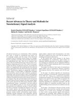
Fig. 2. Space rover simulation system.
3. Camera model
The finite projective camera, which often has pinhole model, is used in this chapter just like
Faugeras suggested (Faugeras and Lustman, 1988). As Fig.3 shows, left and right cameras
have intrinsic parameter matrixes K
q:

0
0
0,1,2
001
uq q q
qvqq
ksu

Kkvq
⎡⎤
⎢⎥
==
⎢⎥
⎢⎥
⎣⎦
(1)
Advances in Theory and Applications of Stereo Vision

116
The subscript q=1,2 denotes left and right camera respectively. If the number of pixels per
unit distance in the image coordinates are m
x
and m
y
in the x and y directions, f is the focal
of length, k
uq
=fm
x
and k
vq
=fm
y
represent the focal length of camera in terms of pixel
dimensions in the x and y directions respectively. S
q
is skew parameter, which is zero for
most normal cameras. However, it is not in some instances like x and y axes is not

perpendicular in the CCD array. u
0q
and v
0q
are the pixel coordinates of image center. The
rotation matrix and translation vector between camera frame F
cq
and world frame F
w
are R
q

and t
q
respectively. A 3D point P projects on image plane. The coordinate transformation
from world reference frame to camera reference frame can be denoted:

cq q w q
PRPt,1,2q
=
+= (2)
The suffix indicates the reference frame, c is camera frame and w is world frame. The
undistorted normalized image projection of P is:

/
/
qcqcq
uq
qcqcq
xXZ

n
yYZ
⎡
⎤⎡ ⎤
==
⎢
⎥⎢ ⎥
⎢
⎥⎢ ⎥
⎣
⎦⎣ ⎦
(3)
P
1C
F
2C
F
1
X
2
X
1
Y
1
Z
2
Y
2
Z
1

p
2
p
W
F

Fig. 3. World frame and camera frames.
As 4mm-focal-length wide angle lens is used in our stereo-vision system, the view angle
approaches 80
o
. In order to improve reconstruction precision, lens distortion must be
considered. Image distortion coefficients are represented by k
1q
, k
2q
, k
3q
, k
4q
and k
5q
. k
1q
, k
2q

and k
5q
denote radial distortion component, and k
3q

, k
4q
denote tangential distortion
component. The distorted image projection n
dq
is the function of the radial distance from the
image center:

2246
125
(1 )
dqqqqqquqq
nkrkrkrndn=+ + + +
(4)
With
222
qqq
rx
y
=+
. dn
q
represents tangential distortion in x and y direction:

22
34
22
34
2(2)
(2)2

qqqqqqq
q
q
qq q qq
dx k x y k r x
dn
dy
kr y kxy
⎡
⎤
++
⎡⎤
⎢
⎥
==
⎢⎥
⎢
⎥
⎢⎥
++
⎣⎦
⎣
⎦
(5)
A High-Precision Calibration Method for Stereo Vision System

117
From (1)(2) and (3), the final distorted pixel coordinate is:
,1,2
qqdq

pKnq
≅
⋅=

(6)
Where ≅ means equal up to a scale factor.
4. Calibration method
The calibration method we use is on the basis of planar homography constraint between the
model plane and its image. The model plane is observed in several positions, just like Zhang
(Z, Z, Zhang, 2000) introduced. At the beginning of calibration, image distortion is not
considered. And the relationship between the 3D point P and its pixel projection p
q
is:

,1,2
qq q q q
pKRtPq
λ
⎡⎤
==
⎣⎦


(7)
Where
q
λ
is an arbitrary factor. We assume the model plane is on Z=0 of the world
coordinate system. Then (6) can be changed into:

qq q
p
HP
λ
=

with
12qqqqq
HKr r t
⎡
⎤
=
⎣
⎦
(8)
Here r
1q
, r
2q
are the first two columns of rotation matrix of two cameras, and H
q
is the planar
homography between two planes. If more than four pairs of corresponding points are
known, H
q
can be computed. Then we can use orthonormal constraint of r
1q
and r
2q
to get

the closed-form solution of intrinsic matrix. Once K
q
is estimated, the extrinsic parameters
,
qq
Rt and the scale factor
q
λ
for each image plane can be easily computed, as Zhang (Z, Z,
Zhang, 2000) indicated.
5. Optimization scheme
As image quantification error exists, the estimated point position and the true value don’t
coincide correctly, especially in z direction. Experiment shows if quantification error reaches
1/4 pixel, the error in z direction may be beyond 1%. Fig.4 shows the observation model
geometrically. Gray ellipses represent uncertainty of 2D image points while the ellipsoids
represent the uncertainty of 3D points. Constant probability contours of the density describe
ellipsoids that approximate the true error density. For nearby points the contours will be close
to spherical; the further the points the more eccentric the coutours become. This illustrates the
importance of modelling the uncertainty by a full 3D Gaussian density, rather than by a single
scalar uncertainty factor. Scalar error models are equivalent to diagonal convariance matrics.
This model is appropriate when 3D points are very close to the camera, but it breaks down
rapidly with increasing distance. Ever though Gaussian error model and uncertainty regions
don’t coincide completely, we still have the opinion Gaussian model will be useful when
quantization error is a significant component of the uncertainty in measured image
coordinates. This uncertainty model is very important in space rover ego-mtion estimation in
space environment when there is no Global Position System(Z, Chuan.& Y, K, Du. 2007).
The above solution in (8) is obtained through minimizing the algebraic distance, which is
not physically meaningful. The commonly used optimization scheme is based on maximum
likelihood estimation:
Advances in Theory and Applications of Stereo Vision

118

2
2
15
111
ˆ
(,,,,,,)
nm
ijq q q q iq iq j
ijq
ppKk kRtP
===
−
∑∑∑
" (9)
Where
15
ˆ
(, ,, , ,,)
qq q
i
q
i
qj
p
Kk k Rt P"
is the estimated projection of point P
j

in image i, followed
by distortion according to (3) and (4). The minimizing process is often solved with LM
Algorithm. However, (8) is not accurate enough if it is used for localization and 3D
reconstruction. The reason is just like section 1 described. Moreover, there are too many
parameters to be estimated, namely, five intrinsic parameters, and five distorted parameters
plus 6n extrinsic parameters for each camera. Each group of extrinsic parameter might be
only optimized for the points on the current plane, while it maybe deviate too much from its
real value. So a new cost function is explored here, which is on the basis of Reconstruction
Error Sum (RES).


Fig. 4. Binocular uncertainty analysis.
5.1 Cost function
Although the cost function using reprojection error is equivalent to maximum likelihood
estimation, it has defect in recovering depth information, for it iteratively adjusts the
estimated parameters to make the estimated image point approach the measured point as
closely as possible. While for 3D points, it may be not. We use Reconstruction Error Sum
(RES) as cost function (Chuan, Long and Gao, 2006):

2
1212
11
() ( , , , )
nm
jijij
ij
RES b P p p b b
==
=−
∑∑

∏
(10)
Where P
j
is a 3D point in the world frame. Its estimated 3D coordinate can be denoted as:
1212
(,,,)
ij ij
p
pbb
∏
, which is reconstructed through triangulation method with given
camera parameters b
1
, b
2
and image projections p
ij1
, p
ij2.
b is a vector consisting 32 calibration
A High-Precision Calibration Method for Stereo Vision System

119
parameters of both left and right cameras, including extrinsic, intrinsic and lens distortion
described in (1), (2), (4), (5):
b={b
1
,b
2

} (11)
b
q
={k
uq
, k
vq
, s
q
, u
0q
, v
0q
, k
1q,
k
2q
, k
3q
, k
4q
, k
5q
, α
q
, β
q
, γ
q
, t

xq
, t
yq
, t
zq
}, q=1,2. And α
q
, β
q
, γ
q
, t
xq
, t
yq
,
t
zq
are rotation angle and translation component between the world frame and camera
frame. So (10) minimizes the sum of all distance between the real 3D points and their
estimated points. This cost function might be better than (9), because (10) is a much stricter
constraint. It exploits the 3D constraint in world frame, while (9) is just a kind of 2D
constraint on image plane. The optimization target P
j
is no bias, because it is assumed to
have no error in 3D space, while p
ijq
in (9) is subject to image quantification error. Even
though (10) still has image quanti-fication error in the image projections, which might
propagate itself to calibration parameter and propagate calibration error to reconstructed 3D

points, the calibration error and the reconstruction error can be reduced by comparing the
3D reconstructed points with their no-bias optimization target P
j
iteratively.
5.2 Searching process
Finding solution b in (11) is a searching process in 32- dimension space. Common
optimization methods like Gauss Newton and LM method might be trapped in local
minimum. Here we use Genetic Algorithms (GA) to search the optimal solution (Gong and
Yang, 2002). GA has been employed with success in variety of problems and it is robust to
local minima and very easy to implement.
The chromosome we construct is b in (11), which has 32 genes. We use real coding because
problems exists in binary encoding, like Hamming Cilff, computing precision and decoding
complexity. The initial parameters of camera calibration are obtained from the methods
introduced in section 3. At the beginning of GA, searching scope must be determined. It is
very important because appropriate searching scope can reduce computational complexity.
The chromosome is generated randomly in the region near the initial value. The fitness
function we chose here is (10). The whole population consists of M individuals, where
M=200. The full description of GA is below:
• Initialization: Generate M individuals randomly. Suppose the generation number t=0, i.e.:
0000
1
{,,,, }
j
M
Gbbb= ""

Where b is chromosome. Superscript is generation number. And subscript denotes
individual number.
• Fitness Computation: Compute fitness value of each chromosome according to (9) and
they are sorted by ascent order, i.e.

11
{,,,, } () ( )
tt t t t t
jM j j
Gb b bandFbFb
+
=≤""

•
Selection operation: Select k individuals according to optimal selection and random
selection.
11 1
1
{,,}
tt t
k
Gb b
+
++
= "
•
Mutation operation: Select p individuals from the new k individuals, and mutate part of
genes randomly.
Advances in Theory and Applications of Stereo Vision

120
11 11 1
11
{,,, ,,}
tt tt t

kk kp
Gb bb b
++ ++ +
++
= ""
•
Crossover operation: Perform crossover operation. Select l genes for crossover
randomly. Repeat it M-k-p times.
11 1 1 1
1
{,,,, ,,}
tt t t t
ikkpM
Gb b b b
+
+++ +
+
= """

•
Let t=t+1. Select the best chromosome as current solution:
1
{ | ( ) min( ( ))}
M
tt t
best i i j
j
b b Fb Fb
=
==

If termination conditions are satisfied, i.e. t is bigger than a predefined number or
()
best
Fb
ε
<
, search process will end. Otherwise, goto step 2.
6. Experiment result
6.1 Simulation experiment result
Both simulation and real image experiments have been done to verify the proposed method.
Both left and right simulated cameras have the following parameter: k
uq
=k
vq
=540, s
q
=0,
u
0q
=400, v
0q
=300, q=1,2. The length of the baseline is 200mm. World frame is bound at the
midpoint on the line connecting the two optic centers. Rotation and translation between two
frames are pre-defined. The distortion parameters of the two cameras are given. Some
emulated points in 3D world, whose distances to the image center are about 1m, project on
the image planes. These image points are added with Gauss noise of different level. With
these image projections and 3D points, we calibrate both emulation cameras with three
different methods, Tsai method, Matlab method (Camera calibration toolbox for matlab),
and our scheme. A normalized error function is defined as:

2
1
ˆ
(1 / )
()
n
ii
i
bb
Eb
n
=
−
=
∑
(12)
It is used to measure the distance between estimated cameras parameters and true cameras
parameters so as to compare the performance of each method. Where
ˆ
,
ii
bb are the i
th

element estimated and real values of (11) respectively, and n is the parameter number of
each method. The performances of three methods are compared, and the results are shown
in table 1, where RES is our method. 1/8, 1/4, and 1/2 pixel noise is added in image points
to verify the robustness of each method. From table 1, it can be seen our method has higher
precision and better robustness than Tsai and Matlab methods.

Tsai Matlab RES
1/8 pixel 1.092 1.245 0.7094
1/4 pixel 1.319 1.597 0.9420
1/2 pixel 2.543 3.001 1.416
Table 1. Normalized error comparison
Scheme
Error

A High-Precision Calibration Method for Stereo Vision System

121
6.2 Real image experiment result
Real image experiment is also performed on the 3D platform, which can translate in X, Y, Z
direction with 1mm precision. The cameras used are IMPERX 2M30, which are working in
the binning mode with 800 600
×
resolution, together with 4mm-focal-length lens. The
length of baseline is 200mm. A calibration chessboard is fixed rigidly on this platform about
1m away from the camera. About 40 images, which are shown in Fig.5, are taken every ten-
centimeter on left, middle and right side of view field along depth direction. The
configuration between the camers and chessboard is shown in Fig.6. First we use all the
corner points as control points for coarse calibration. Then 4 points of each image, altogether
about 160 points are selected for optimization with (10). The rest 7000 points are used for
verification. We use Pentium 1.7GHz CPU, and VC++ 6.0 developing environment,
calibration process needs about 30 minutes. Calibration result obtained from Tsai method,
Matlab toolbox and our scheme, are used to reconstruct these points. Error distribution
histogram is shown in Fig.7, in which (a) is Tsai method, (b) is Matlab scheme, and (c) is our
RES method. The unit of horizontal axis is millimeter. Table 2 shows statistic reconstruction

errors along X, Y, Z direction, including mean error A(X), A(Y), A(Z), maximal error M(X),


Fig. 5. All calibration images of left camera.

Fig. 6. Chessboard and cameras configration.
Advances in Theory and Applications of Stereo Vision

122
M(Y), M(Z), and variance , ,
xyz
σ
σσ
. From these figures and table, it can be seen our
scheme can have much higher precision than other method, especially in depth direction.



Tsai Matlab RES
A(X)
2.3966 3.4453 1.7356
A(Y)
2.1967 2.2144 1.6104
A(Z)
4.2987 5.2509 2.3022
M(X)
9.5756 13.6049 5.7339
M(Y)
9.8872 12.5877 7.3762
M(Z)

15.1088 19.1929 7.3939
σ
x

2.4499 2.7604 1.7741
σ
y

2.3873 3.0375 1.8755
σ
z

4.7211 4.8903 2.4063
Table 2. Statistic error comparison

(a)

(b)

(c)
Fig. 7. Reconstruction error distribution comparison. (a) Tsai method. (b) Matlab method. (c)
RES method.
Scheme
Error
A High-Precision Calibration Method for Stereo Vision System

123
6.3 Real environment experiment result
In order to validate the calibration precision in real application, we set up a 15×20m indoor
environment, and a 6×3m slope made up of sand and rock. We calibrate the navigation

cameras, which have 8mm-focal-length lens, in the way introduced above. After the images
are captured, as Fig.8 shows, we perform character extraction, point match, 3D point-cloud
creation. DEM and triangle grids are generated using these 3D points. Then the gray levels
of the images are mapped to the virtual environment graphics. Finally, we have the virtual
simulational environment, as Fig.9 indicates, which is highly consistent with the real
environment. The virtual space rover is put into this environment for path planning and
validation. In Fig.10, the blue line, which is the planned path, is generated by operator. The
simulation rover follows this path to detect if there is any collision. If not, the operator
transmitts this instruction to space rover to execute.
In order to validate the calibration precision for arm operation in real environment, we set
up a board in front of the rover arm. The task of the rover arm is to drill the board, collect
sample and analyse its component. We calibrate the hazard detection cameras, which have
4mm-focal-length lens, in the way introduced above too. After the images are captured, as
Fig.11 shows, we perform character extraction, point match, 3D point-cloud creation. DEM
and triangle grids are generated using these 3D points. The virtual simulation environment,
as Fig.12 indicates, can be generated in the same way as mentioned above. The virtual space
rover together with its arm, which has 5 degree of freedom, are put into this environment

for trajectory planning and validation. After the opertor interactively gives a drill point on
the board, the simalation system calculates whether point is within or out of the arm work
space. Or there is any collision and singularity configuration on the trajectory. This process
repeats until it proves to be safe. Then the operator transmitts this instruction to the rover
arm to execute. Both of the experients prove the calibration precision is accurate enough for
rover navigation and arm operation.


Fig. 8. Image captured by navigation camera.
Advances in Theory and Applications of Stereo Vision

124

(a)



(b)

Fig. 9. Virtual simulation environment. (a) Gray mapping frame. (b) Grid frame.
A High-Precision Calibration Method for Stereo Vision System

125







Fig. 10. Path planning for simulation rover.








Fig. 11. Image captured by hazard detection camera.

Advances in Theory and Applications of Stereo Vision

126






Fig. 12. Drill operation simulation for rover arm
7. Conclusion
Stereo vision can percept and measure the 3-D information of the unstructured environment
in a passive manner. It provides consultant support for robotics control and decision-
making, and it can be applied in the field of rover navigation, real-time hazard avoidance,
path programming and terrain modelling. In this chapter, a high precision camera
calibration method is proposed for stereo vision system in space rover using wide angle
lens. It exploits 5 parameters to describe lens distortion. To alleviate the problems in the
existing calibration techniques, we develop an alternative paradigm based on a new cost
function to conventional reprojection error cost function. Genetic algorithm is used in
searching process in order to get globally optimal solution in high-dimension parameter
space and avoid trapping in local minimum instead of differential method. Simulation and
real images experiments show that this scheme has higher precision and better robustness
than traditional method for space localization. In real envrionment experiment, both Digital
Elevation Map and virtual simulation environment can be generated accurately for rover
path planning, validation and arm operation. It can be successfully used in space rover
simulation system.
8. Acknowledgement
This research is supported by the National High-Technology 863 Program (Grant No.
2004AA420090).
A High-Precision Calibration Method for Stereo Vision System

127
9. References
Murry, D.& Jennings C. (1997). “Stereo vision based mapping and navigation for mobile
robots”, In: Proceedings of IEEE Conference on Robotics and Automation, pp.1694- 1699.
R, Y, Tsai. (1987). “A versatile camera calibration technique for high-accuracy 3d machine
vision metrology using off-the shelf tv cameras and lenses,” IEEE Journal of Robotics
and Automation, vol.3, no.4, pp.323-344.
J, Yunde.; L. Hongjing,; X. An,& L. Wanchun. (2000). “Fish-Eye Lens Camera Calibration for
Stereo Vision System”, Chinese Journal of Computers, vol.23, no.11, pp.1215-1219.
Camera calibration toolbox for matlab, web site:
/calib_doc/.
D, B, Gennery. (2001). “Least-squares camera calibration includeing lens distortion and
automatic editing of calibration points”, Calibration and Orien-tation of Cameras in
Computer Vision, T. Huang, Springer-Verlag, New York.
Z, Z, Zhang. (2000). “A flexible new technique for camera calibration,” IEEE Transactions on
Pattern Analysis and Machine Intelligence, vol.22, no. 11, pp. 1330- 1334.
M, L, Gong.& Y. H. Yang. (2002). “Genetic-based stereo algorithm and disparity map
evaluation,” International Journal of Computer Vision, vol.47, no.1, pp.63-77.
Z, Chuan.; T, D, Long.& Z, Feng. (2004). “A High- Precision Calibration Method for
Distorted Camera.” IROS, Sep 28-Oct 2, Sendai, Japan, pp.2618- 2623.
T. S. Huang, A. N. Arun, “Motion and structure from feature correspondences: a review,”
Proceedings of the IEEE, vol.82, no.2, 1994, pp.252-268.
J. Weng, P. Cohen, and M. Herniou, “Camera calibration with distortion models and
accuracy evaluation,” IEEE Transaction on Pattern Analysis and Machine Intelligence,
vol.14, no.10, 1992, pp. 965-980.
Z, Chuan.; T, D, Long. & H, W, Gao. (2006). “A High-Precision Calibration and Optimization
Method for Stereo Vision System.“ International Conference on Control, Automation,
Robotics and Vision, Singapore, 5-8th December, pp.1158-1162.
Z, Chuan.; T, D, Long.& Z. Feng. (2004). “A High-Precision Binocular Method for Model-

Based Pose Estimation“, International Conference on Control, Automation, Robotics and
Vision, Kunming, China, 6-9th December, pp.1067-1071.
Z, Chuan.& Y, K, Du. (2007). “A motion estimation method based on binocular recon-
struction uncertainty analysis. “ Chinese Journal of Science Instrument (in Chinese).
Vol.4, pp.15-17.
Z, Chuan.; T, D, Long.; Z, F,& D, Z, Li. (2003). “A Planar Homography Estimation Method
for Camera Calibration.“ IEEE International Symposium on Computational Intelligence
in Robotics and Automation, Kobe, Japan, pp.424-429.
C, F, Olson.; L, H, Matthies.; M, Schoppers.& M, W, Maimone. (2003). “Rover navigation
using stereo ego-motion“. Robotics and Autonomous Systems, 2003, vol.43, pp.215-
229.
R, Hartley.& A, Zisserman. (2001). “Multiple View Geometry in Computer Vision.”
Cambridge University Press.
Y. L. Xiong.; C, F, Olson.& L, H, Matthies. (2001). “Computing Depth Maps From Descent
Imagery.” Proceedings of the IEEE Computer Society Conference on Computer Vision and
Pattern Recongnition, Kauai, Hawaii, Dec, Vol.1, pp. 392-397.
P, G, Backes.& K, S, Tso. (1999). “The Web Interface for Telescience.” Presence, vol.8, No.5,
pp.531-529.
Advances in Theory and Applications of Stereo Vision

128
M, A, Vona.& P, G, Backes.; J, S, Norris.& M, W, Powell. “Challenges in 3D Visualization for
Mars Exploration Rover Mission Science Planning.”
S, B, Goldberg.; M, W, Maimone.& L, Matthies. (2002). “Stereo Vision and Rover Navigation
Software for Planetary Exploration.” IEEE Aerospace Conference Proceedings, March,
Big Sky, Montana, USA, pp.
O, Faugeras.& F, Lustman. (1988). “Motion and structure from motion in a piecewise planar
environment“. International Journal of Pattern Recognition and Artificial Intelligence.
2(3), pp.485-508.
E, Malis.& R, Cipolla. (2000). “Multi-view constraints between collineations: application to

self-calibration from unknown planar structures“. European Conference on Computer
Vision, vol.2, Dublin, Ireland, pp.610-624.
M, Muhlich.& R, Mester. (1998). “The role of total least squares in motion analysis“.
European Conference on Computer Vision, pp. 305-321.
M, Muhlich.& R, Mester. “The subspace method and equilibration in computer vision“.
Technical report XP-TR-C-21
0
Stereo Correspondence with Local Descriptors for
Object Recognition
Gee-Sern Jison Hsu
National Taiwan University of Science and Technology
Taiwan
1. Introduction
Stereo correspondence refers to the matches between two images with different viewpoints
looking at the same object or scene. It is one of the most active research topics in computer
vision as it plays a central role in 3D object recognition, object categorization, view synthesis,
scene reconstruction, and many other applications. The image pair with different viewpoints
is known as stereo images when the baseline and camera parameters are given. Given
stereo images, the approaches for finding stereo correspondences are generally split into two
categories: one based on sparse local features found matched between the images, and the
other based on dense pixel-to-pixel matched regions found between the images. The former
is proven effective for 3D object recognition and categorization, while the latter is better for
view synthesis and scene reconstruction. This chapter focuses on the former because of the
increasing interests in 3D object recognition in recent years, also because the feature-based
methods have recently made a substantial progress by several state-of-the-art local (feature)
descriptors.
The study of object recognition using stereo vision often requires a training set which offers
stereo images for developing the model for each object considered, and a test set which
offers images with variations in viewpoint, scale, illumination, and occlusion conditions for
evaluating the model. Many methods on local descriptors consider each image from stereo

or multiple views a single instance without exploring much of the relationship between these
instances, ending up with models of multiple independent instances. Using such a model for
object recognition is like matching between a training image and a test image. It is, however,
especially interested in this chapter that models are developed integrating the information
across multiple training images. The central concern is how to extract local features from
stereo or multiple images so that the information from different views can be integrated in
the modeling phase, and applied in the recognition phase. This chapter is composed of the
following contents:
1. Affine invariant region detection in Section 2: Many invariant image features are
proposed in the last decade. Because these features are invariant to image variations in
viewpoint, scale, illumination, and other variables, they serve well for establishing stereo
correspondences across images. Those with better invariance to viewpoint changes are of
special interest as they can be of direct use in the development of object models from stereo
or multi-view.
7
2 Stereo Vision
2. Local region descriptors in Section 3: These descriptors transform affine invariant regions
into vectors or distributions so that some distance measure can be applied to discern the
similarity or difference between features. Again, those with better invariance to viewpoint
changes are especially interested.
3. Object modeling and recognition using local region descriptors from multi-view in Section
4: A couple methods are reviewed that develop models by combining the information from
local descriptors extracted across multiple views. These methods offer good examples on
how to integrate local invariant features across different views.
4. A case study on performance evaluation and benchmark databases in Section 5:
Implementation of others’ methods for performance comparison with one’s own proposed
method takes a tremendous amount of time and efforts. Therefore, a database commonly
accepted for performance benchmark is needed, and different methods can be evaluated
on the same testbed. A performance evaluation example is reviewed with an introduction
on its database, followed by a snapshot on other databases also good for study on 3D object

recognition using stereo correspondences.
2. Affine regions for stereo correspondence
Affine-invariant region detectors can identify the affine-invariant regions on multiple images
which are the projections of the same 3D surface patches. The regions are also considered
as covariant with geometric and photometric transformations, as the regions detected in one
image can be mapped onto those detected in the other using these transformations. Different
affine detectors give different local regions in terms of different locations, sizes, orientations
and the numbers of detected regions.
Mikolajczyk et al. (2005) have evaluated six affine region detectors, including Harris-affine,
Hessian-affine, edge-based region, intensity extrema-based region, salient region and
maximally stable extremal region (MSER). This evaluation focuses on the performance of
matching between two images with variations caused by viewpoint, scale, illumination, blur
and JPEG compression. The detectors for regions only covariant to similarity transform
are excluded in their evaluation, for example the interest regions extracted to develop the
Scale-Invariant Feature Transform (SIFT) by Lowe (1999; 2004) and the scale invariant features
by Mikolajczyk & Schmid (2001). However, the SIFT descriptor (Lowe, 1999; 2004) is used in
this evaluation to characterize the intensity patterns of the regions detected by the above six
detectors.
The scope of this chapter is on finding stereo correspondences for object recognition, subject
to the requirement that the object’s model is built on at least a pair of stereo images with
different viewpoints. In certain cases, the objects in stereo or multiple images may appear
slightly different in scale. Therefore the detectors that perform better than others in rendering
correct matches under viewpoint and scale changes are of special interest in this chapter. This
performance can be justified by the repeatability and matching score from the evaluation in
Mikolajczyk et al. (2005). It is shown that the Harris-affine detector, Hessian-affine detector
and the maximally stable extremal region (MSER) detector are three promising ones in offering
reliable stereo correspondences under viewpoint and scale changes. Note that illumination
changes, blur and JPEG compression are among the major challenging parameters when
recognizing a test image, the three aforementioned detectors also perform well when testing
against these parameters, as revealed by Mikolajczyk et al. (2005).

130
Advances in Theory and Applications of Stereo Vision
Stereo Correspondence with Local Descriptors for Object Recognition 3
2.1 Harris and hessian affine detectors
Harris affine region detector exploits a combination of Harris corner detector, Gaussian
scale-space and affine shape adaptation. The core part is based on the following second
moment matrix,
M
(x,σ
D
,σ
I
)=σ
2
D
G(σ
I
) ∗

L
2
x
(x,σ
D
) L
x
L
y
(x,σ
D

)
L
x
L
y
(x,σ
D
) L
2
y
(x,σ
D
)

(1)
where L
(˙, σ
D
) is the image smoothed by a Gaussian kernel with differentiation scale σ
D
;
L
x
(x,σ
D
) and L
y
(x,σ
D
) are the first derivatives of the image along x− and y− directions,

respectively, at point x. The derivatives are then averaged in a neighborhood of x by
convolving with G
(σ
I
), a Gaussian filter with integration scale σ
I
. The eigenvalues of
M
(x,σ
D
,σ
I
) measure the changes of the gradients along two orthogonal directions in that
neighborhood region. When the change is larger than a threshold, the region is considered a
corner-like feature in the image.
Fig. 1. Scale invariant interest point detection in affine transformed images: (Top) Initial
interest points detected by multi-scale Harris detector with characteristic scales selected by
Laplacian scale peak (in black–Harris-Laplace). (Bottom) Characteristic point detected with
Harris-Laplace (in black) and the corresponding point from the other image projected with
the affine transformation (in white). Reproduced from Mikolajczyk & Schmid (2004).
Given an image, the algorithm for detecting Harris affine regions consists of the following
steps (Mikolajczyk & Schmid, 2002; 2004; Mikolajczyk et al., 2005):
131
Stereo Correspondence with Local Descriptors for Object Recognition
4 Stereo Vision
1. Detection of scale-invariant interest regions using the Harris-Laplace detector and a characteristic
scale selection scheme: Given σ
I
and σ
D

, the scale-adapted Harris corner detector using the
second moment matrix M in (1) can be used to estimate corner-like features. To determine
the characteristic scale, σ
∗
I
, the scale-adapted Harris corner is first applied with a number
of preselected scales, resulting in corners in multiple scales. Given these corners, the
algorithm given by Lindeberg (1998) can be applied, which iteratively searches for both the
characteristic scale σ
∗
I
and the spatial location x
∗
that maximize the Laplacian-of-Gaussians
(LoG) over the preselected scales.
2. Normalization of the scale-invariant interest regions obtained in Step 1 using Affine Shape
Adaptation: The obtained scale-invariant interest regions are normalized using affine shape
adaptation (Lindeberg & G
˚
arding, 1997), which again uses the second moment matrix M in
(1) but generalized with non-uniform Gaussian kernels for anisotropic regions (versus the
uniform Gaussian kernels in (1) for isotropic regions). It is an extension of the regular
scale-space obtained by convolution with rotationally symmetric Gaussian kernels to an
affine Gaussian scale-space obtained by shape-adapted Gaussian kernels. This step results in
initial estimates on the affine regions.
3. Iterative estimation of the affine region: The step in each iterative loop are composed of the
generation of a reference frame using a shape adaptation matrix U
(k−1)
, the selection of an
appropriate integration scale σ

(k)
I
and differentiation scale σ
(k)
D
, and the spatial localization
of an interest point x
(k)
, where ·
(k)
denotes for the k-th iteration. The shape adaptation
matrix is the concatenation of square roots of the second moment matrices and is often
initialized by the identity matrix. The integration scale is selected at the maximum over
a predefined range of scales of the normalized Laplacian, and the differentiation scale is
selected at the maximum of normalized isotropy. To reduce complexity, Mikolajczyk &
Schmid (2002; 2004) make σ
D
= sσ
I
, where s is a constant factor between 0.5 to 0.75.
4. Affine region update using the updated scales, σ
(k)
I
and σ
(k)
I
, and spatial localizations x
(k)
.
This allows the second moment matrix M

(k)
renewed, and the shape adaptation matrix
U
(k)
updated.
5. Return to Step 3 if the stopping criterion on the isotropy measure is not met. Because the
above algorithm in each iterative loop searches for the shape adaptation matrix U
(k)
that
transforms an anisotropic region into an isotropic region, the iteration terminates when the
ratio between the minimum and maximum eigenvalues of M
(k)
becomes sufficiently close
to 1.
Fig. 1, reproduced from Mikolajczyk & Schmid (2004), shows an example from initial
estimates of the regions using multi-scale Harris detector to the final affine invariant regions.
In addition to the above Harris-Affine region detector based on the Harris-Laplace detector
in (1), a similar alternative is Hessian-Affine region detector based on the Hessian matrix
(Mikolajczyk et al., 2005),
H
(x,σ
D
)=

L
xx
(x,σ
D
) L
xy

(x,σ
D
)
L
xy
(x,σ
D
) L
xx
(x,σ
D
)

(2)
According to Mikolajczyk et al. (2005), the second derivatives, L
xx
, L
xy
and L
xy
give strong
responses on blobs and ridges. The scheme is similar to the blob detection given by Lindeberg
(1998). The points maximizing the determinant of the Hessian matrix will penalize long
132
Advances in Theory and Applications of Stereo Vision
Stereo Correspondence with Local Descriptors for Object Recognition 5
structures with small second derivatives in one particular orientation. A local maximum of
the determinant indicates the presence of a blob. The detection of Hessian-Affine regions
is almost the same as the iterative algorithm for Harris-Affine regions, but with the second
moment matrix in (1) replaced by the Hessian matrix in (2). Fig. 2, given in Mikolajczyk et al.

(2005), shows examples of Harris-Affine and Hessian-Affine regions.
(a) Harris-Affine
(b) Hessian-Affine
Fig. 2. Examples of regions detected by Harris-Affine and Hessian-Affine detectors;
reproduced from Mikolajczyk et al. (2005)
2.2 Maximally stable extremal region (MSER)
MSER is proposed by Matas et al. (2002) to find correspondences between two images of
different viewpoints. The extraction of MSER considers the set of all possible thresholds able
to binarize an intensity image I
(x) into a binary image E
t
M
(x),
E
t
M
(x)=

1 ifI
(x) ≤ t
M
0 otherwise.
(3)
where t
M
is the threshold. A MSER is a connected region in E
t
M
(x) with little change in its size
for a range of thresholds. The number of thresholds that maintain the connected region similar

in size is known as the margin of the region. One can successively increase the threshold t
M
in (3) to detect dark regions, denoted as MSER+; or invert the intensity image first and then
increase the threshold to detect bright regions, denoted as MSER An example given by
Forss
´
en & Lowe (2007) with margin larger than 7 is shown in Fig. 3.
Because it is defined exclusively by the intensity function in the region and the outer border,
and the local binarization is stable over a large range of thresholds, the MSER possesses the
following characteristics which make it favorable in many cases (Matas et al., 2002; Nist
´
er &
Stew
´
enius, 2008):
133
Stereo Correspondence with Local Descriptors for Object Recognition
6 Stereo Vision
Fig. 3. Regions detected by a MSER with margin 7, reproduced from Forss
´
en & Lowe (2007).
– The regions are closed under continuous (and thus projective) transformation of image
coordinates, indicating that they are affine invariant regardless if the image is warped or
skewed.
– The regions are closed under monotonic transformation of image intensities, reflecting that
photometric changes have no effect on these regions, so they are robust to illumination
variations.
– The regions are stable because their support is virtually unchanged over a range of
thresholds.
– The detection performs across multiple scales without any smoothing involved, so both fine

and large structures are discovered. If it operates with a scale pyramid, the repeatability and
the number of correspondences across scales can be further improved.
– The set of all extremal regions can be enumerated in worst-case O
(n), where n is the number
of pixels in the image.
Besides, the extensive performance evaluation by Mikolajczyk et al. (2005) shows the
following characteristics of MSER:
– Viewpoint change: MSER outperforms other detectors in both the original images and those
with repeated texture motifs.
– Scale change: MSER is outperformed by the Hessian-Affine detector only, in the
repeatability percentage and matching score when the scale factor is large than 2.
– Illumination change: MSER gives the highest repeatability percentage.
– Region size - MSER appears to render more small regions than many others do, and small
interest regions can be better in recognizing objects with occlusion.
– Blur - The performance of MSER degrades substantially when blur increases, and therefore,
other detectors should be considered when recognizing objects in blur images. This might
be the only variable that MSER cannot handle well.
134
Advances in Theory and Applications of Stereo Vision
Stereo Correspondence with Local Descriptors for Object Recognition 7
MSER has been extended to color images by Forss
´
en & Lowe 2007. This extension studies
successive time-steps of an agglomerative clustering of color pixels. The selection of
time-steps is stabilized against intensity scalings and image blur by modeling the distribution
of edge magnitudes. The algorithm contains an edge significance measure based on a Poisson
image noise model, yielding a better performance than the original MSER from Matas et al.
(2002), especially when extracting such interest regions from color images.
3. Local region descriptors
Local region descriptors are mostly in vector forms that can characterize the pattern of

an interest point with its neighboring region. Ten different descriptors are reviewed and
evaluated by Mikolajczyk & Schmid (2005), including the scale invariant feature transform
(SIFT) by Lowe (2004), gradient location and orientation histogram (GLOH) by Mikolajczyk
& Schmid (2005), shape context (Belongie et al., 2002), PCA-SIFT (Ke & Sukthankar, 2004),
spin images (Lazebnik et al., 2003), steerable filters (Freeman & Adelson, 1991), differential
invariants (Koenderink & van Doom, 1987), complex filters (Schaffalitzky & Zisserman,
2002), moment invariants (Gool et al., 1996) , and cross-correlation of sampled pixel values
(Mikolajczyk & Schmid, 2005). Five region detectors are used to offer interest regions
in this evaluation study: Harris corners, Harris-Laplace regions, Hessian-Laplace regions,
Harris-Affine regions and Hessian-Affine regions. Given an image, these detectors are first
applied to identify interest regions, which are used to compute the descriptors.
Similar to the previous section that selects the affine invariant regions good for handling
viewpoint and scale variations, this section focuses on the region descriptors good for the
same variables. Fig. 4, reproduced from Mikolajczyk & Schmid (2005), shows a few
comparisons on viewpoint and scale changes in terms of 1
−precision versus recall.1−precision
and recall are defined as follows:
1
− precision =
N
f
N
c
+ N
f
(4)
rec all
=
N
c

N
cr
(5)
where N
c
and N
f
are the numbers of correct and false matches, respectively, and both change
with the threshold that measures the distance between descriptors. N
cr
is the number of
correspondences. N
c
and N
cr
depend on the overlap error, which measures how well the
corresponding regions fit each other under homography transformation. A perfect descriptor
would give a unity recall for any precision. In practice, recall increases with decreasing
precision (and thus increasing 1
−precision). For any fixed precision, the descriptors that yield
higher recalls are more desirable.
It can be seen that GLOH (Mikolajczyk & Schmid, 2005) performs the best, closely followed by
SIFT (Lowe, 2004) and shape context (Belongie et al. 2002) in generating more correct matches
under viewpoint and scale changes. Actually, as revealed by the extensive experimental study
in Mikolajczyk & Schmid (2005), these three descriptors also outperform the others in most
tests with other variables.
3.1 SIFT and GLOH descriptors
SIFT (Scale-Invariant Feature Transform) descriptor, proposed by Lowe (2004), is derived
from a 3D histogram of gradient location and orientation. GLOH (Gradient Location and
135

Stereo Correspondence with Local Descriptors for Object Recognition
8 Stereo Vision
(a) Viewpoint change with structured scene
and Hessian-Affine regions
(b) Viewpoint change with textured scene
and Hessian-Affine regions
(c) Scale change with structured scene and
Hessian-Laplace regions
(d) Scale change with textured scene and
Hessian-Laplace regions
Fig. 4. Performance comparison of region descriptors for viewpoint and scale changes,
reproduced from Mikolajczyk & Schmid (2005).
Orientation Histogram) is a modified version of SIFT, given by Mikolajczyk & Schmid (2005),
which computes a SIFT descriptor for a log-polar location grid with bins in both radial and
angular directions.
Figs. 5a and 5b summarizes the computation of a SIFT descriptor. The gradient magnitudes
and orientations are first computed at each sample point in a region around an interest point
(or keypoint as called in Lowe, 2004), as the arrows shown in Fig. 5a. Each arrow shows the
magnitude of the gradient by its length, and the orientation by its arrowhead. A Gaussian
blur window, shown by the blue circle in Fig. 5a, is imposed on the interest region with σ
equal to one half the width of the region’s scale, assigning a weight to the magnitude of each
sample point. This Gaussian window can avoid sudden changes in the descriptor with small
perturbations on the position of the region, and weaken the contribution from the gradients far
from the center of the region. Fig. 5a shows a 2
×2 descriptor array with 4 subregions inside,
and each subregion is formed by 4
× 4 elements. The gradients in each subregion can be
segmented according to the eight major orientations, and summed up in magnitude for each
orientation, transforming the 8
×8 gradient patterns to the 2×2 descriptor patterns, as shown

in Fig. 5b. This 2
×2 descriptor pattern gives a vector of 2×2 ×8 = 32 in dimension. However,
136
Advances in Theory and Applications of Stereo Vision
Stereo Correspondence with Local Descriptors for Object Recognition 9
Fig. 5. (a) 2 ×2 descriptor array with 4 subregions inside, and each subregion is formed by
4
×4 elements. The gradients are smoothed by a Gaussian window shown in blue circle. (b)
The 8 orientation bins in each subregion can be combined with bins from other subregions,
leading to a vector descriptor for this interest region.
based on the experiments by Lowe (2004), the best descriptor that has been exhaustively tested
is with 4
×4 array, leading to a descriptor vector of 4 ×4 × 8 = 128 in dimension. To obtain
illumination invariance, this descriptor is normalized by the square root of the sum of squared
components.
GLOH is SIFT descriptor computed for a log-polar location grid with three spatial elements
in radial direction (with radius 6, 11, and 15) and eight orientations. Only the subregion with
smallest radius is not segmented to orientations, and this gives 2
× 8 + 1 = 17 subregion in
total. The gradient orientations in each subregion are quantized into 16 bins, and this gives
to the interest region a vector of 272 in dimension. PCA (Principal Component Analysis) is
then applied to downsize its dimension to 128 using the principal components extracted from
47,000 patches collected from various images. The experiments in Mikolajczyk & Schmid
(2005) reveal that GLOH performs slightly better than SIFT in many tests.
3.2 Shape context descriptor
Shape context, proposed by Belongie et al. (2002), is a descriptor that characterize the shape
of an object. Given a shape, which can be obtained by an edge detector, one can pick a point
p
i
out of the n points on the shape and compute the histogram h

i
of the relative coordinates of
the remaining n
−1 points,
h
i
(k)=#{q = p
i
: (q − p
i
) ∈ bin (k)} (6)
where k denotes for the k-th bin of the histogram, q denotes a point on the shape. This
histogram, measured in a log-polar space, defines the shape context descriptor of p
i
. It reveals
the distribution of the shape relative to p
i
in terms of log(r) and θ, where r measures the
distance and θ measures the orientation. This design makes the descriptor more sensitive to
the locations of nearby shape points than to those farther apart. Belongie et al. (2002), use 5
bins for log
(r) and 12 bins for θ, giving a descriptor of dimension 60; while in Mikolajczyk
& Schmid (2005), r is split into 9 bins with θ in 4 bins, resulting in a descriptor of dimension
36. Fig.6, from Belongie et al. (2002), shows an example of shape context computation and
matching.
Given a point p
i
on the first shape and a point q
i
on the second shape, C

ij
, which denotes the
cost of matching these two points, can be computed using their shape context descriptors as
137
Stereo Correspondence with Local Descriptors for Object Recognition
10 Stereo Vision
(a) (b) (c)
(d) (e) (f) (g)
Fig. 6. Shape context computation and matching, (a) and (b) are the sampled edge points of
two ”A” shapes. (c) Diagram of log-polar histogram bins used for computing shape contexts,
5 bins for logr and 12 for θ. (d), (e) and (f) are the shape contexts obtained for the reference
points marked by
◦, , and , respectively. Similar patterns between ◦ and , and a different
one at
 can be observed. (g) Correspondences found by bipartite matching. All are
reproduced from Belongie et al. 2002.
follows,
C
ij
≡ C(p
i
,q
j
)=
1
2
K
∑
k=1
|h

i
(k) − h
j
(k)|
2
h
i
(k)+h
j
(k)
(7)
where h
i
(k) and h
j
(k) denote the K-bin normalized histogram at p
i
and q
j
, respectively. (7)
applies the χ
2
test for measuring the difference between distributions. The total cost of
matching all point pairs can then be written as
H
(π)=
∑
i
C(p
i

,q
π(i)
) (8)
where π is a permutation to be determined to minimize H
(π). This is a typical case
in weighted bipartite matching problem, which can be solved in O
(N
3
) time using the
Hungarian algorithm (Papadimitriou and Stieglitz, 1982).
Minimization of H
(π) over π gives the correspondences at the sample points. The
correspondence is extended to the complete shape using the regularized thin plate splines
as the aligning transform. Aligning shapes leads to a general measure of shape similarity.
The dissimilarity between two shapes can thus be computed as the sum of matching errors
between corresponding points. Given this dissimilarity measure, Belongie et al. (2002), apply
nearest-neighbor algorithms for object recognition.
138
Advances in Theory and Applications of Stereo Vision