david roylance mechanics of materials Part 6 ppt
Bạn đang xem bản rút gọn của tài liệu. Xem và tải ngay bản đầy đủ của tài liệu tại đây (509.51 KB, 25 trang )
Constitutive Equations
David Roylance
Department of Materials Science and Engineering
Massachusetts Institute of Technology
Cambridge, MA 02139
October 4, 2000
Introduction
The modules on kinematics (Module 8), equilibrium (Module 9), and tensor transformations
(Module 10) contain concepts vital to Mechanics of Materials, but they do not provide insight on
the role of the material itself. The kinematic equations relate strains to displacement gradients,
and the equilibrium equations relate stress to the applied tractions on loaded boundaries and also
govern the relations among stress gradients within the material. In three dimensions there are
six kinematic equations and three equilibrum equations, for a total of nine. However, there are
fifteen variables: three displacements, six strains, and six stresses. We need six more equations,
and these are provided by the material’s consitutive relations: six expressions relating the stresses
to the strains. These are a sort of mechanical equation of state, and describe how the material
is constituted mechanically.
With these constitutive relations, the vital role of the material is reasserted: The elastic
constants that appear in this module are material properties, subject to control by processing
and microstructural modification as outlined in Module 2. This is an important tool for the
engineer, and points up the necessity of considering design of the material as well as with the
material.
Isotropic elastic materials
In the general case of a linear relation between components of the strain and stress tensors, we
might propose a statement of the form
ij
= S
ijkl
σ
kl
where the S
ijkl
is a fourth-rank tensor. This constitutes a sequence of nine equations, since each
component of
ij
is a linear combination of all the components of σ
ij
. For instance:
23
= S
2311
σ
11
+ S
2312
σ
12
+ ···+S
2333
33
Based on each of the indices of S
ijkl
taking on values from 1 to 3, we might expect a total of 81
independent components in S. However, both
ij
and σ
ij
are symmetric, with six rather than
nine independent components each. This reduces the number of S components to 36, as can be
seen from a linear relation between the pseudovector forms of the strain and stress:
1
x
y
z
γ
yz
γ
xz
γ
xy
=
S
11
S
12
··· S
16
S
21
S
22
··· S
26
.
.
.
.
.
.
.
.
.
.
.
.
S
61
S
26
··· S
66
σ
x
σ
y
σ
z
τ
yz
τxz
τ
xy
(1)
It can be shown
1
that the S matrix in this form is also symmetric. It therefore it contains only
21 independent elements, as can be seen by counting the elements in the upper right triangle of
the matrix, including the diagonal elements (1 + 2 + 3 + 4 + 5 + 6 = 21).
If the material exhibits symmetry in its elastic response, the number of independent elements
in the S matrix can be reduced still further. In the simplest case of an isotropic material, whose
stiffnesses are the same in all directions, only two elements are independent. We have earlier
shown that in two dimensions the relations between strains and stresses in isotropic materials
can be written as
x
=
1
E
(σ
x
− νσ
y
)
y
=
1
E
(σ
y
− νσ
x
)
γ
xy
=
1
G
τ
xy
(2)
along with the relation
G =
E
2(1 + ν)
Extending this to three dimensions, the pseudovector-matrix form of Eqn. 1 for isotropic mate-
rials is
x
y
z
γ
yz
γ
xz
γ
xy
=
1
E
−ν
E
−ν
E
000
−ν
E
1
E
−ν
E
000
−ν
E
−ν
E
1
E
000
000
1
G
00
0000
1
G
0
00000
1
G
σ
x
σ
y
σ
z
τ
yz
τxz
τ
xy
(3)
The quantity in brackets is called the compliance matrix of the material, denoted S or S
ij
.It
is important to grasp the physical significance of its various terms. Directly from the rules of
matrix multiplication, the element in the i
th
row and j
th
column of S
ij
is the contribution of the
j
th
stress to the i
th
strain. For instance the component in the 1,2 position is the contribution
of the y-direction stress to the x-direction strain: multiplying σ
y
by 1/E gives the y-direction
strain generated by σ
y
, and then multiplying this by −ν gives the Poisson strain induced in
the x direction. The zero elements show the lack of coupling between the normal and shearing
components.
The isotropic constitutive law can also be written using index notation as (see Prob. 1)
ij
=
1+ν
E
σ
ij
−
ν
E
δ
ij
σ
kk
(4)
where here the indicial form of strain is used and G has been eliminated using G = E/2(1 + ν)
The symbol δ
ij
is the Kroenecker delta, described in the Module on Matrix and Index Notation.
1
G.M. Mase, Schaum’s Outline of Theory and Problems of Continuum Mechanics, McGraw-Hill, 1970.
2
If we wish to write the stresses in terms of the strains, Eqns. 3 can be inverted. In cases of
plane stress (σ
z
= τ
xz
= τ
yz
= 0), this yields
σ
x
σ
y
τ
xy
=
E
1 − ν
2
1 ν 0
ν 10
00(1−ν)/2
x
y
γ
xy
(5)
where again G has been replaced by E/2(1 + ν). Or, in abbreviated notation:
σ = D (6)
where D = S
−1
is the stiffness matrix.
Hydrostatic and distortional components
Figure 1: Hydrostatic compression.
A state of hydrostatic compression, depicted in Fig. 1, is one in which no shear stresses exist
and where all the normal stresses are equal to the hydrostatic pressure:
σ
x
= σ
y
= σ
z
= −p
where the minus sign indicates that compression is conventionally positive for pressure but
negative for stress. For this stress state it is obviously true that
1
3
(σ
x
+ σ
y
+ σ
z
)=
1
3
σ
kk
= −p
so that the hydrostatic pressure is the negative mean normal stress. This quantity is just one
third of the stress invariant I
1
, which is a reflection of hydrostatic pressure being the same in
all directions, not varying with axis rotations.
In many cases other than direct hydrostatic compression, it is still convenient to “dissociate”
the hydrostatic (or “dilatational”) component from the stress tensor:
σ
ij
=
1
3
σ
kk
δ
ij
+Σ
ij
(7)
Here Σ
ij
is what is left over from σ
ij
after the hydrostatic component is subtracted. The Σ
ij
tensor can be shown to represent a state of pure shear, i.e. there exists an axis transformation
such that all normal stresses vanish (see Prob. 5). The Σ
ij
is called the distortional, or deviatoric,
3
component of the stress. Hence all stress states can be thought of as having two components as
shown in Fig. 2, one purely extensional and one purely distortional. This concept is convenient
because the material responds to these stress components is very different ways. For instance,
plastic and viscous flow is driven dominantly by distortional components, with the hydrostatic
component causing only elastic deformation.
Figure 2: Dilatational and deviatoric components of the stress tensor.
Example 1
Consider the stress state
σ =
567
689
792
,GPa
The mean normal stress is σ
kk
/3=(5+8+2)/3 = 5, so the stress decomposition is
σ =
1
3
σ
kk
δ
ij
+Σ
ij
=
500
050
005
+
06 7
63 9
79−3
It is not obvious that the deviatoric component given in the second matrix represents pure shear, since
there are nonzero components on its diagonal. However, a stress transformation using Euler angles
ψ = φ =0,θ =−9.22
◦
gives the stress state
Σ
=
0.00 4.80 7.87
4.80 0.00 9.49
7.87 9.49 0.00
The hydrostatic component of stress is related to the volumetric strain through the modulus
of compressibility (−p = K ∆V/V), so
1
3
σ
kk
= K
kk
(8)
Similarly to the stress, the strain can also be dissociated as
ij
=
1
3
kk
δ
ij
+ e
ij
where e
ij
is the deviatoric component of strain. The deviatoric components of stress and strain
are related by the material’s shear modulus:
Σ
ij
=2Ge
ij
(9)
4
where the factor 2 is needed because tensor descriptions of strain are half the classical strains
for which values of G have been tabulated. Writing the constitutive equations in the form of
Eqns. 8 and 9 produces a simple form without the coupling terms in the conventional E-ν form.
Example 2
Using the stress state of the previous example along with the elastic constants for steel (E = 207 GPa,ν =
0.3,K = E/3(1 − 2ν) = 173 GPa,G = E/2(1 + ν)=79.6 Gpa), the dilatational and distortional
components of strain are
δ
ij
kk
=
δ
ij
σ
kk
3K
=
0.0289 0 0
00.0289 0
000.0289
e
ij
=
Σ
ij
2G
=
00.0378 0.0441
0.0378 0.0189 0.0567
0.0441 0.0567 −0.0189
The total strain is then
ij
=
1
3
kk
δ
ij
+ e
ij
=
0.00960 0.0378 0.0441
0.0378 0.0285 0.0567
0.0441 0.0567 −0.00930
If we evaluate the total strain using Eqn. 4, we have
ij
=
1+ν
E
σ
ij
−
ν
E
δ
ij
σ
kk
=
0.00965 0.0377 0.0440
0.0377 0.0285 0.0565
0.0440 0.0565 −0.00915
These results are the same, differing only by roundoff error.
Finite strain model
When deformations become large, geometrical as well as material nonlinearities can arise that
are important in many practical problems. In these cases the analyst must employ not only a
different strain measure, such as the Lagrangian strain described in Module 8, but also different
stress measures (the “Second Piola-Kirchoff stress” replaces the Cauchy stress when Lagrangian
strain is used) and different stress-strain constitutive laws as well. A treatment of these for-
mulations is beyond the scope of these modules, but a simple nonlinear stress-strain model
for rubbery materials will be outlined here to illustrate some aspects of finite strain analysis.
The text by Bathe
2
provides a more extensive discussion of this area, including finite element
implementations.
In the case of small displacements, the strain
x
is given by the expression:
x
=
1
E
[σ
x
− ν(σ
y
+ σ
z
)]
For the case of elastomers with ν =0.5, this can be rewritten in terms of the mean stress
σ
m
=(σ
x
+σ
y
+σ
z
)/3as:
2
x
=
3
E
(σ
x
−σ
m
)
2
K J. Bathe, Finite Element Procedures in Engine ering Analysis, Prentice-Hall, 1982.
5
For the large-strain case, the following analogous stress-strain relation has been proposed:
λ
2
x
=1+2
x
=
3
E
(σ
x
−σ
∗
m
) (10)
where here
x
is the Lagrangian strain and σ
∗
m
is a parameter not necessarily equal to σ
m
.
The σ
∗
m
parameter can be found for the case of uniaxial tension by considering the transverse
contractions λ
y
= λ
z
:
λ
2
y
=
3
E
(σ
y
− σ
∗
m
)
Since for rubber λ
x
λ
y
λ
z
=1,λ
2
y
=1/λ
x
. Making this substitution and solving for σ
∗
m
:
σ
∗
m
=
−Eλ
2
y
3
=
−E
3λ
x
Substituting this back into Eqn. 10,
λ
2
x
=
3
E
σ
x
−
E
3λ
x
Solving for σ
x
,
σ
x
=
E
3
λ
2
x
−
1
λ
x
Here the stress σ
x
= F/A is the “true” stress based on the actual (contracted) cross-sectional
area. The “engineering” stress σ
e
= F/A
0
based on the original area A
0
= Aλ
x
is:
σ
e
=
σ
x
λ
x
= G
λ
x
−
1
λ
2
x
where G = E/2(1 + ν)=E/3forν=1/2. This result is the same as that obtained in Module
2 by considering the force arising from the reduced entropy as molecular segments spanning
crosslink sites are extended. It appears here from a simple hypothesis of stress-strain response,
using a suitable measure of finite strain.
Anisotropic m aterials
Figure 3: An orthotropic material.
If the material has a texture like wood or unidirectionally-reinforced fiber composites as
shown in Fig. 3, the modulus E
1
in the fiber direction will typically be larger than those in the
transverse directions (E
2
and E
3
). When E
1
= E
2
= E
3
, the material is said to be orthotropic.
6
It is common, however, for the properties in the plane transverse to the fiber direction to be
isotropic to a good approximation (E
2
= E
3
); such a material is called transversely isotropic.
The elastic constitutive laws must be modified to account for this anisotropy, and the following
form is an extension of Eqn. 3 for transversely isotropic materials:
1
2
γ
12
=
1/E
1
−ν
21
/E
2
0
−ν
12
/E
1
1/E
2
0
001/G
12
σ
1
σ
2
τ
12
(11)
The parameter ν
12
is the principal Poisson’s ratio; it is the ratio of the strain induced in the
2-direction by a strain applied in the 1-direction. This parameter is not limited to values less
than 0.5 as in isotropic materials. Conversely, ν
21
gives the strain induced in the 1-direction by
a strain applied in the 2-direction. Since the 2-direction (transverse to the fibers) usually has
much less stiffness than the 1-direction, it should be clear that a given strain in the 1-direction
will usually develop a much larger strain in the 2-direction than will the same strain in the
2-direction induce a strain in the 1-direction. Hence we will usually have ν
12
>ν
21
.Thereare
five constants in the above equation (E
1
, E
2
, ν
12
, ν
21
and G
12
). However, only four of them are
independent; since the S matrix is symmetric, ν
21
/E
2
= ν
12
/E
1
.
A table of elastic constants and other properties for widely used anisotropic materials can
be found in the Module on Composite Ply Properties.
The simple form of Eqn. 11, with zeroes in the terms representing coupling between normal
and shearing components, is obtained only when the axes are aligned along the principal material
directions; i.e. along and transverse to the fiber axes. If the axes are oriented along some other
direction, all terms of the compliance matrix will be populated, and the symmetry of the material
will not be evident. If for instance the fiber direction is off-axis from the loading direction, the
material will develop shear strain as the fibers try to orient along the loading direction as shown
in Fig. 4. There will therefore be a coupling between a normal stress and a shearing strain,
which never occurs in an isotropic material.
Figure 4: Shear-normal coupling.
The transformation law for compliance can be developed from the transformation laws for
strains and stresses, using the procedures described in Module 10 (Transformations). By suc-
cessive transformations, the pseudovector form for strain in an arbitrary x-y direction shown in
Fig. 5 is related to strain in the 1-2 (principal material) directions, then to the stresses in the 1-2
directions, and finally to the stresses in the x-y directions. The final grouping of transformation
matrices relating the x-y strains to the x-y stresses is then the transformed compliance matrix
7
Figure 5: Axis transformation for constitutive equations.
in the x-y direction:
x
y
γ
xy
= R
x
y
1
2
γ
xy
= RA
−1
1
2
1
2
γ
12
= RA
−1
R
−1
1
2
γ
12
= RA
−1
R
−1
S
σ
1
σ
2
τ
12
= RA
−1
R
−1
SA
σ
x
σ
y
τ
xy
≡ S
σ
x
σ
y
τ
xy
where S is the transformed compliance matrix relative to x-y axes. Here A is the transformation
matrix, and R is the Reuter’s matrix defined in the Module on Tensor Transformations. The
inverse of
S is D, the stiffness matrix relative to x-y axes:
S = RA
−1
R
−1
SA, D = S
−1
(12)
Example 3
Consider a ply of Kevlar-epoxy composite with a stiffnesses E
1
= 82, E
2
=4,G
12
=2.8(allGPa)and
ν
12
=0.25. The compliance matrix S in the 1-2 (material) direction is:
S =
1/E
1
−ν
21
/E
2
0
−ν
12
/E
1
1/E
2
0
001/G
12
=
.1220 × 10
−10
−.3050 × 10
−11
0
−.3050 × 10
−11
.2500 × 10
−9
0
00.3571 × 10
−9
If the ply is oriented with the fiber direction (the “1” direction) at θ =30
◦
from the x-y axes, the
appropriate transformation matrix is
A =
c
2
s
2
2sc
s
2
c
2
−2sc
−sc sc c
2
− s
2
=
.7500 .2500 .8660
.2500 .7500 −.8660
−.4330 .4330 .5000
The compliance matrix relative to the x-y axes is then
S = RA
−1
R
−1
SA =
.8830 × 10
−10
−.1970 × 10
−10
−.1222 × 10
−9
−.1971 × 10
−10
.2072 × 10
−9
−.8371 × 10
−10
−.1222 × 10
−9
−.8369 × 10
−10
−.2905 × 10
−9
Note that this matrix is symmetric (to within numerical roundoff error), but that nonzero coupling
values exist. A user not aware of the internal composition of the material would consider it completely
anisotropic.
8
The apparent engineering constants that would be observed if the ply were tested in the x-y rather
than 1-2 directions can be found directly from the trasnformed
S matrix. For instance, the apparent
elastic modulus in the x direction is E
x
=1/S
1,1
=1/(.8830 × 10
−10
)=11.33 GPa.
Problems
1. Expand the indicial forms of the governing equations for solid elasticity in three dimensions:
equilibrium : σ
ij,j
=0
kinematic :
ij
=(u
i,j
+ u
j,i
)/2
constitutive :
ij
=
1+ν
E
σ
ij
−
ν
E
δ
ij
σ
kk
+ αδ
ij
∆T
where α is the coefficient of linear thermal expansion and ∆T is a temperature change.
2. (a) Write out the compliance matrix S of Eqn. 3 for polycarbonate using data in the
Module on Material Properties.
(b) Use matrix inversion to obtain the stiffness matrix D.
(c) Use matrix multiplication to obtain the stresses needed to induce the strains
=
x
y
z
γ
yz
γ
xz
γ
xy
=
0.02
0.0
0.03
0.01
0.025
0.0
3. (a) Write out the compliance matrix S of Eqn.3 for an aluminum alloy using data in the
Module on Material Properties.
(b) Use matrix inversion to obtan the stiffness matrix D.
(c) Use matrix multiplication to obtain the stresses needed to induce the strains
=
x
y
z
γ
yz
γ
xz
γ
xy
=
0.01
0.02
0.0
0.0
0.15
0.0
4. Given the stress tensor
σ
ij
=
123
245
357
(MPa)
(a) Dissociate σ
ij
into deviatoric and dilatational parts Σ
ij
and (1/3)σ
kk
δ
ij
.
9
(b) Given G = 357 MPa and K =1.67 GPa, obtain the deviatoric and dilatational strain
tensors e
ij
and (1/3)
kk
δ
ij
.
(c) Add the deviatoric and dilatational strain components obtained above to obtain the
total strain tensor
ij
.
(d) Compute the strain tensor
ij
using the alternate form of the elastic constitutive law
for isotropic elastic solids:
ij
=
1+ν
E
σ
ij
−
ν
E
δ
ij
σ
kk
Compare the result with that obtained in (c).
5. Provide an argument that any stress matrix having a zero trace can be transformed to one
having only zeroes on its diagonal; i.e. the deviatoric stress tensor Σ
ij
represents a state
of pure shear.
6. Write out the x-y two-dimensional compliance matrix
S and stiffness matrix D (Eqn. 12)
for a single ply of graphite/epoxy composite with its fibers aligned along the x axes.
7. Write out the x-y two-dimensional compliance matrix
S and stiffness matrix D (Eqn. 12)
for a single ply of graphite/epoxy composite with its fibers aligned 30
◦
from the x axis.
10
Statics of Bending: Shear and Bending Moment Diagrams
David Roylance
Department of Materials Science and Engineering
Massachusetts Institute of Technology
Cambridge, MA 02139
November 15, 2000
Introduction
Beams are long and slender structural elements, differing from truss elements in that they are
called on to support transverse as well as axial loads. Their attachment points can also be
more complicated than those of truss elements: they may be bolted or welded together, so the
attachments can transmit bending moments or transverse forces into the beam. Beams are
among the most common of all structural elements, being the supporting frames of airplanes,
buildings, cars, people, and much else.
The nomenclature of beams is rather standard: as shown in Fig. 1, L is the length, or span;
b is the width, and h is the height (also called the depth). The cross-sectional shape need not
be rectangular, and often consists of a vertical web separating horizontal flanges at the top and
bottom of the beam
1
.
Figure 1: Beam nomenclature.
As will be seen in Modules 13 and 14, the stresses and deflections induced in a beam under
bending loads vary along the beam’s length and height. The first step in calculating these quan-
tities and their spatial variation consists of constructing shear and bending moment diagrams,
V (x)andM(x), which are the internal shearing forces and bending moments induced in the
beam, plotted along the beam’s length. The following sections will describe how these diagrams
are made.
1
Figure 2: A cantilevered beam.
Free-body diagrams
As a simple starting example, consider a beam clamped (“cantilevered”) at one end and sub-
jected to a load P at the free end as shown in Fig. 2. A free body diagram of a section cut
transversely at position x shows that a shear force V and a moment M must exist on the cut
section to maintain equilibrium. We will show in Module 13 that these are the resultants of shear
and normal stresses that are set up on internal planes by the bending loads. As usual, we will
consider section areas whose normals point in the +x direction to be positive; then shear forces
pointing in the +y direction on +x faces will be considered positive. Moments whose vector
direction as given by the right-hand rule are in the +z direction (vector out of the plane of the
paper, or tending to cause counterclockwise rotation in the plane of the paper) will be positive
when acting on +x faces. Another way to recognize positive bending moments is that they cause
the bending shape to be concave upward. For this example beam, the statics equations give:
F
y
=0=V +P⇒V = constant = −P (1)
M
0
=0=−M+Px⇒M =M(x)=Px (2)
Note that the moment increases with distance from the loaded end, so the magnitude of the
maximum value of M compared with V increases as the beam becomes longer. This is true of
most beams, so shear effects are usually more important in beams with small length-to-height
ratios.
Figure 3: Shear and bending moment diagrams.
1
There is a standardized protocol for denoting structural steel beams; for instance W 8 × 40 indicates a
wide-flange beam with a nominal depth of 8
and weighing 40 lb/ft of length
2
As stated earlier, the stresses and deflections will be shown to be functions of V and M,soit
is important to be able to compute how these quantities vary along the beam’s length. Plots of
V (x)andM(x) are known as shear and bending moment diagrams, and it is necessary to obtain
them before the stresses can be determined. For the end-loaded cantilever, the diagrams shown
in Fig. 3 are obvious from Eqns. 1 and 2.
Figure 4: Wall reactions for the cantilevered beam.
It was easiest to analyze the cantilevered beam by beginning at the free end, but the choice
of origin is arbitrary. It is not always possible to guess the easiest way to proceed, so consider
what would have happened if the origin were placed at the wall as in Fig. 4. Now when a free
body diagram is constructed, forces must be placed at the origin to replace the reactions that
were imposed by the wall to keep the beam in equilibrium with the applied load. These reactions
can be determined from free-body diagrams of the beam as a whole (if the beam is statically
determinate), and must be found before the problem can proceed. For the beam of Fig. 4:
F
y
=0=−V
R
+P ⇒V
R
=P
M
o
=0=M
R
−PL ⇒M
R
= PL
The shear and bending moment at x are then
V (x)=V
R
=P = constant
M(x)=M
R
−V
R
x=PL−Px
This choice of origin produces some extra algebra, but the V (x)andM(x) diagrams shown in
Fig. 5 are the same as before (except for changes of sign): V is constant and equal to P ,andM
varies linearly from zero at the free end to PL at the wall.
Distributed loads
Transverse loads may be applied to beams in a distributed rather than at-a-point manner as
depicted in Fig. 6, which might be visualized as sand piled on the beam. It is convenient to
describe these distributed loads in terms of force per unit length, so that q(x) dx would be the
load applied to a small section of length dx by a distributed load q(x). The shear force V (x)set
up in reaction to such a load is
V (x)=−
x
x
0
q(ξ)dξ (3)
3
Figure 5: Alternative shear and bending moment diagrams for the cantilevered beam.
Figure 6: A distributed load and a free-body section.
where x
0
is the value of x at which q(x)begins,andξis a dummy length variable that looks
backward from x. Hence V (x) is the area under the q(x) diagram up to position x. The moment
balance is obtained considering the increment of load q(ξ) dξ applied to a small width dξ of beam,
adistanceξfrom point x. The incremental moment of this load around point x is q(ξ) ξdξ,so
the moment M(x)is
M=
x
x
0
q(ξ)ξdξ (4)
This can be related to the centroid of the area under the q(x) curve up to x, whose distance
from x is
¯
ξ =
q(ξ) ξdξ
q(ξ)dξ
Hence Eqn. 4 can be written
M = Q
¯
ξ (5)
where Q =
q(ξ) dξ is the area. Therefore, the distributed load q(x) is statically equivalent to
a concentrated load of magnitude Q placed at the centroid of the area under the q(x) diagram.
Example 1
Consider a simply-supported beam carrying a triangular and a concentrated load as shown in Fig. 7. For
4
Figure 7: Distributed and concentrated loads.
the purpose of determining the support reaction forces R
1
and R
2
, the distributed triangular load can be
replaced by its static equivalent. The magnitude of this equivalent force is
Q =
2
0
(−600x) dx = −1200
The equivalent force acts through the centroid of the triangular area, which is is 2/3 of the distance from
its narrow end (see Prob. 1). The reaction R
2
can now be found by taking moments around the left end:
M
A
=0=−500(1) − (1200)(2/3) + R
2
(2) → R
2
= 650
The other reaction can then be found from vertical equilibrium:
F
y
=0=R
1
−500 − 1200 + 650 = 1050
Successive integration method
Figure 8: Relations between distributed loads and internal shear forces and bending moments.
We have already noted in Eqn. 3 that the shear curve is the negative integral of the loading
curve. Another way of developing this is to consider a free body balance on a small increment
5
of length dx over which the shear and moment changes from V and M to V + dV and M + dM
(see Fig. 8). The distributed load q(x) can be taken as constant over the small interval, so the
force balance is:
F
y
=0=V +dV + qdx−V =0
dV
dx
= −q
(6)
or
V (x)=−
q(x)dx (7)
which is equivalent to Eqn. 3. A moment balance around the center of the increment gives
M
o
=(M+dM)+(V +dV )
dx
2
+ V
dx
2
− M
As the increment dx is reduced to the limit, the term containing the higher-order differential
dV dx vanishes in comparison with the others, leaving
dM
dx
= −V
(8)
or
M(x)=−
V(x)dx (9)
Hence the value of the shear curve at any axial location along the beam is equal to the negative
of the slope of the moment curve at that point, and the value of the moment curve at any point
is equal to the negative of the area under the shear curve up to that point.
The shear and moment curves can be obtained by successive integration of the q(x) distri-
bution, as illustrated in the following example.
Example 2
Consider a cantilevered beam subjected to a negative distributed load q(x)=−q
0
=constant as shown
in Fig. 9; then
V (x)=−
q(x)dx = q
0
x + c
1
where c
1
is a constant of integration. A free body diagram of a small sliver of length near x =0shows
that V (0) = 0, so the c
1
must be zero as well. The moment function is obtained by integrating again:
M(x)=−
V(x)dx = −
1
2
q
0
x
2
+ c
2
where c
2
is another constant of integration that is also zero, since M(0) = 0.
Admittedly, this problem was easy because we picked one with null boundary conditions, and
with only one loading segment. When concentrated or distributed loads are found at different
6
Figure 9: Shear and moment distributions in a cantilevered beam.
positions along the beam, it is necessary to integrate over each section between loads separately.
Each integration will produce an unknown constant, and these must be determined by invoking
the continuity of slopes and deflections from section to section. This is a laborious process, but
one that can be made much easier using singularity functions that will be introduced shortly.
It is often possible to sketch V and M diagrams without actually drawing free body dia-
grams or writing equilibrium equations. This is made easier because the curves are integrals or
derivatives of one another, so graphical sketching can take advantage of relations among slopes
and areas.
These rules can be used to work gradually from the q(x)curvetoV(x) and then to M(x).
Wherever a concentrated load appears on the beam, the V (x) curve must jump by that value,
but in the opposite direction; similarly, the M(x) curve must jump discontinuously wherever a
couple is applied to the beam.
Example 3
Figure 10: A simply supported beam.
To illustrate this process, consider a simply-supported beam of length L as shown in Fig. 10, loaded
7
over half its length by a negative distributed load q = −q
0
. The solution for V (x)andM(x)takesthe
following steps:
1. The reactions at the supports are found from static equilibrium. Replacing the distributed load
by a concentrated load Q = −q
0
(L/2) at the midpoint of the q distribution (Fig. 10(b))and taking
moments around A:
R
B
L =
q
0
L
2
3L
4
⇒R
B
=
3q
0
L
8
The reaction at the right end is then found from a vertical force balance:
R
A
=
q
0
L
2
− R
B
=
q
0
L
8
Note that only two equilibrium equations were available, since a horizontal force balance would
provide no relevant information. Hence the beam will be statically indeterminate if more than two
supports are present.
The q(x) diagram is then just the beam with the end reactions shown in Fig. 10(c).
2. Beginning the shear diagram at the left, V immediately jumps down to a value of −q
0
L/8in
opposition to the discontinuously applied reaction force at A; it remains at this value until x = L/2
as shown in Fig. 10(d).
3. At x = L/2, the V (x) curve starts to rise with a constant slope of +q
0
as the area under the q(x)
distribution begins to accumulate. When x = L, the shear curve will have risen by an amount
q
0
L/2, the total area under the q(x) curve; its value is then (−q
0
l/8) + (q
0
L/2) = (3q
0
L/8). The
shear curve then drops to zero in opposition to the reaction force R
B
=(3q
0
L/8). (The V and M
diagrams should always close, and this provides a check on the work.)
4. The moment diagram starts from zero as shown in Fig. 10(e), since there is no discontinuously
applied moment at the left end. It moves upward at a constant slope of +q
0
L/8, the value of the
shear diagram in the first half of the beam. When x = L/2, it will have risen to a value of q
0
L
2
/16.
5. After x = L/2, the slope of the moment diagram starts to fall as the value of the shear diagram
rises. The moment diagram is now parabolic, always being one order higher than the shear diagram.
The shear diagram crosses the V = 0 axis at x =5L/8, and at this point the slope of the moment
diagram will have dropped to zero. The maximum value of M is 9q
0
L
2
/32, the total area under
the V curve up to this point.
6. After x =5L/8, the moment diagram falls parabolically, reaching zero at x = L.
Singularity functions
This special family of functions provides an automatic way of handling the irregularities of
loading that usually occur in beam problems. They are much like conventional polynomial
factors, but with the property of being zero until “activated” at desired points along the beam.
The formal definition is
f
n
(x)=x−a
n
=
0,x<a
(x−a)
n
,x>a
(10)
where n = −2, −1, 0, 1, 2, ···. The function x − a
0
is a unit step function, x − a
−1
is a
concentrated load, and x − a
−2
is a concentrated couple. The first five of these functions are
sketched in Fig. 11.
8
Figure 11: Singularity functions.
The singularity functions are integrated much like conventional polynomials:
x
−∞
x − a
n
dx =
x − a
n+1
n +1
n≥0 (11)
However, there are special integration rules for the n = −1andn=−2 members, and this
special handling is emphasized by using subscripts for the n index:
x
−∞
x − a
−2
dx = x − a
−1
(12)
x
−∞
x − a
−1
dx = x − a
0
(13)
Example 4
Applying singularity functions to the beam of Example 4.3, the loading function would be written
q(x)=+
q
0
L
8
x−0
−1
−q
0
x−
L
2
0
The reaction force at the right end could also be included, but it becomes activated only as the problem
is over. Integrating once:
V (x)=−
q(x)dx = −
q
0
L
8
x
0
+ q
0
x −
L
2
1
The constant of integration is included automatically here, since the influence of the reaction at A has
been included explicitly. Integrating again:
M(x)=−
V(x)dx =
q
0
L
8
x
1
−
q
0
2
x −
L
2
2
Examination of this result will show that it is the same as that developed previously.
Maple
TM
symbolic manipulation software provides an efficient means of plotting these functions. The
following shows how the moment equation of this example might be plotted, using the Heaviside function
to provide the singularity.
9
# Define function sfn in terms of a and n
>sfn:=proc(a,n) (x-a)^n*Heaviside(x-a) end;
sfn := proc(a, n) (x - a)^n*Heaviside(x - a) end proc
# Input moment equation using singularity functions
>M(x):=(q*L/8)*sfn(0,1)-(q/2)*sfn(L/2,2);
M(x) := 1/8qLxHeaviside(x)
2
- 1/2 q (x - 1/2 L) Heaviside(x - 1/2 L)
# Provide numerical values for q and L:
>q:=1: L:=10:
# Plot function
>plot(M(x),x=0 10);
Figure 12: Maple singularity plot
Problems
1. (a)–(c) Locate the magnitude and position of the force equivalent to the loading distribu-
tions shown here.
2. (a)–(c) Determine the reaction forces at the supports of the cases in Prob. 1.
3. (a)–(h) Sketch the shear and bending moment diagrams for the load cases shown here.
4. (a)–(h) Write singularity-function expressions for the shear and bending moment distribu-
tions for the cases in Prob. 3.
5. (a)–(h) Use Maple (or other) software to plot the shear and bending moment distributions
for the cases in Prob. 3, using the values (as needed) L =25in,a=5in,w =10lb/in,P =
150 lb.
10
Prob. 1
Prob. 3
6. The transverse deflection of a beam under an axial load P is taken to be δ(y)=δ
0
sin(yπ/L),
as shown here. Determine the bending moment M(y)alongthebeam.
7. Determine the bending moment M(θ) along the circular curved beam shown.
11
Prob. 6
Prob. 7
12
STRESSES IN BEAMS
David Roylance
Department of Materials Science and Engineering
Massachusetts Institute of Technology
Cambridge, MA 02139
November 21, 2000
Introduction
Understanding of the stresses induced in beams by bending loads took many years to develop.
Galileo worked on this problem, but the theory as we use it today is usually credited principally
to the great mathematician Leonard Euler (1707–1783). As will be developed below, beams
develop normal stresses in the lengthwise direction that vary from a maximum in tension at
one surface, to zero at the beam’s midplane, to a maximum in compression at the opposite
surface. Shear stresses are also induced, although these are often negligible in comparision
with the normal stresses when the length-to-height ratio of the beam is large. The procedures
for calculating these stresses for various loading conditions and beam cross-section shapes are
perhaps the most important methods to be found in introductory Mechanics of Materials, and
will be developed in the sections to follow. This theory requires that the user be able to construct
shear and bending moment diagrams for the beam, as developed for instance in Module 12.
Normal Stresses
A beam subjected to a positive bending moment will tend to develop a concave-upward curva-
ture. Intuitively, this means the material near the top of the beam is placed in compression along
the x direction, with the lower region in tension. At the transition between the compressive and
tensile regions, the stress becomes zero; this is the neutral axis of the beam. If the material
tends to fail in tension, like chalk or glass, it will do so by crack initiation and growth from
the lower tensile surface. If the material is strong in tension but weak in compression, it will
fail at the top compressive surface; this might be observed in a piece of wood by a compressive
buckling of the outer fibers.
We seek an expression relating the magnitudes of these axial normal stresses to the shear
and bending moment within the beam, analogously to the shear stresses induced in a circular
shaft by torsion. In fact, the development of the needed relations follows exactly the same direct
approach as that used for torsion:
1. Geometrical statement: We begin by stating that originally transverse planes within the
beam remain planar under bending, but rotate through an angle θ about points on the
neutral axis as shown in Fig. 1. For small rotations, this angle is given approximately by
1
the x-derivative of the beam’s vertical deflection function v(x)
1
:
u = −yv
,x
(1)
where the comma indicates differentiation with respect to the indicated variable (v
,x
≡
dv/dx). Here y is measured positive upward from the neutral axis, whose location within
the beam has not yet been determined.
Figure 1: Geometry of beam bending.
2. Kinematic equation: The x-direction normal strain
x
is then the gradient of the displace-
ment:
x
=
du
dx
= −yv
,xx
(2)
Note that the strains are zero at the neutral axis where y = 0, negative (compressive)
above the axis, and positive (tensile) below. They increase in magnitude linearly with y,
much as the shear strains increased linearly with r in a torsionally loaded circular shaft.
The quantity v
,xx
≡ d
2
v/dx
2
is the spatial rate of change of the slope of the beam deflection
curve, the “slope of the slope.” This is called the curvature of the beam.
3. Constitutive equation: The stresses are obtained directly from Hooke’s law as
σ
x
= E
x
= −yEv
,xx
(3)
This restricts the applicability of this derivation to linear elastic materials. Hence the
axial normal stress, like the strain, increases linearly from zero at the neutral axis to a
maximum at the outer surfaces of the beam.
4. Equilibrium relations: Since there are no axial (x-direction) loads applied externally to the
beam, the total axial force generated by the normal σ
x
stresses (shown in Fig. 2) must be
zero. This can be expressed as
1
The exact expression for curv ature is
dθ
ds
=
d
2
v/dx
2
[1 + (dv/dx)
2
]
3/2
This gives θ ≈ dv/dx when the squared derivative in the denominator is small compared to 1.
2
F
x
=0=
A
σ
x
dA =
A
−yEv
,xx
dA
which requires that
A
ydA=0
The distance ¯y from the neutral axis to the centroid of the cross-sectional area is
¯y =
A
ydA
A
dA
Hence ¯y = 0, i.e. the neutral axis is coincident with the centroid of the beam cross-sectional
area. This result is obvious on reflection, since the stresses increase at the same linear rate,
above the axis in compression and below the axis in tension. Only if the axis is exactly
at the centroidal position will these stresses balance to give zero net horizontal force and
keep the beam in horizontal equilibrium.
Figure 2: Moment and force equilibrium in the beam.
The normal stresses in compression and tension are balanced to give a zero net horizontal
force, but they also produce a net clockwise moment. This moment must equal the value
of M(x)atthatvalueofx, as seen by taking a moment balance around point O:
M
O
=0=M+
A
σ
x
·ydA
M =
A
(yEv
,xx
) · ydA=Ev
,xx
A
y
2
dA (4)
Figure 3: Moment of inertia for a rectangular section.
3