Encyclopedia of Smart Materials (Vols 1 and 2) - M. Schwartz (2002) WW Part 15 pps

P1: FCH/FYX P2: FCH/FYX QC: FCH/UKS T1: FCH
PB091-V-Drv January 10, 2002 21:38
VIBRATION CONTROL IN SHIP STRUCTURES 1101
Table 1. Advantages and Disadvantages of Various Sensor and Actuator Technologies
Type of Sensor or Actuator Advantages Disadvantages
Piezoelectric materials
Examples:
Lead zirconate
Titanate (PZT)
Polyvinylidene
Fluoride(PVDF)
r
Used as sensors and actuators
r
Relatively low strain and low displacement
r
Very large frequency range capability (typically, less than 0.1% strain,
r
Quick response time and 1–100 microns displacement for
r
Very high resolution and dynamic range stack actuators)
r
Possibility of integration in the structure
r
Actuators require relatively costly
for thin PZT actuators and PVDF voltage amplifiers
sensors
r
Low recoverable strain (0.1%)
r

Possibility of shaping PVDF sensors
r
Piezoelectric ceramics are brittle
(spatial filtering)
r
Cannot measure direct current
r
Susceptible to high hysteresis
and creep when strained in direction
of poling (e.g., stack actuators)
Electrostrictive
materials
Example:
Lead-magnesium
niobate (PMN)
r
Used as sensor and actuators
r
More sensitive to temperature
r
Lower hysteresis and creep variations than piezoelectrics
compared to piezoelectric
r
Potentially larger recoverable strain
than piezoelectric
Magnetostrictive
materials
Example:
Terfenol-D
r

Higher force and strain capability than
r
Low recoverable strain (0.15%)
piezoceramics (typically, 1000
r
Only for compression components
microstrain deformation)
r
Nonlinear behavior
r
Suited for high-precision applications
r
Suited for compressive load carrying
components
r
Very durable
Shape-memory alloys
(SMA)
Example:
NITINOL
r
Large recoverable strain (8%)
r
Suited for low-frequency (0–10 Hz)
used largely for actuation due to large and low-precision application
force generation
r
Slow response time
r
Low voltage requirements

r
Complex constitutive behavior
with large hysteresis
Optical fibers
Examples:
Bragg grating,
Fabry-Perot
r
Suited for remote sensing of structures
r
Used for sensing alone
r
Corrosion resistant
r
Behavior is complicated by thermal strains
r
Immune to electric interference
r
Small, light, and compatible with
advanced composite
Electrorheological
fluids (ER)
Example:
Alumino-silicate
in paraffin oil
r
Simple and quiet devices
r
Low-frequency applications
r

Suitable for vibration control
r
Nonlinear behavior
r
Offers significant capability and
r
Cannot tolerate impurities
flexibility for altering structural response
r
Fluid and solid phases tend to separate
r
Low density
r
Not suitable for low temperature applications
r
High-voltage requirements (2–10 kV)
r
Higher η
p
/τ
2
y
ratio than MR*
Magnetorheological
r
Simple and quiet devices
r
Nonlinear behavior
fluids (MR)
r

Quick response time
r
Higher density than ER
r
Suitable for vibration control
r
Offers significant capability and
flexibility for altering structural response
r
Low voltage requirements
r
Behavior not affected by impurities
r
Suitable for wide range of temperatures
r
Lower η
p
/τ
2
y
ratio than ER*
Microphones
r
Low cost
r
Sensitive to turbulent flow
r
Large dynamic range
r
Need to achieve directionality in

r
Excellent linearity some active control systems (e.g., ducts)
r
Need protection to dust,
moisture, high temperature
(cont.)
P1: FCH/FYX P2: FCH/FYX QC: FCH/UKS T1: FCH
PB091-V-Drv January 10, 2002 21:38
1102 VIBRATION CONTROL IN SHIP STRUCTURES
Table 1. (Continued.)
Type of Sensor or Actuator Advantages Disadvantages
Displacement sensors
Example:
Proximity probe,
LVDT, LVIT
r
Good low-frequency sensitivity (0–10 Hz)
r
Low-frequency range (typically, below 100 Hz)
r
Noncontacting measurement (proximity probe)
r
Low dynamic range (typically, 100 : 1)
r
Well suited to measurement of relative
r
Low resolution
displacement in active mounts
Velocity sensors
r

Noncontacting measurement
r
Low dynamic range (typically 100 : 1)
(magnetic)
r
Well suited to measurement of relative
r
Low resolution
velocity in active mounts
r
Heavy
Accelerometers
r
Large dynamic range
r
Low sensitivity in low frequency (0–10 Hz)
r
Excellent linearity
r
Require relatively expensive charge
amplifiers (piezoelectric accelerometers)
Loudspeakers
r
Low cost
r
Nonlinear behavior if driven close to maximum power
r
Space requirement (backing enclosure)
r
Need protection to dust, moisture, high

temperature, corrosive environment
Electrodynamic and
r
Relatively large force/large
r
May need a large reaction mass to
electromagnetic displacement capability transmit large forces
actuators
r
Excellent linearity
r
Space requirement
r
Extended frequency range
Hydraulic and
r
Large force/large
r
Low-frequency range (0–10 Hz for
pneumatic actuators displacement capability pneumatic; 0–150 Hz for hydraulic)
r
Need for hydraulic or compressed air power supply
r
Nonlinear behavior
r
Space requirement
in an annular armature. When the coil is activated, the
TERFENOL rod expands and produces a displacement.
The TERFENOL-D bar, coil, and armature are assem-
bled between two steel washers and put inside a protec-

tive wrapping to form the basic magnetoactive induced
strain actuator unit (7). The main advantage of terfenol is
its high-force capability at relatively low cost (21). It also
has the advantage of small size and light weight, which
makes it suitable for situations where no reactive mass is
required such as in stiffened structures of aircraft and sub-
marine hulls. The disadvantages of TERFENOL include
its brittleness and low tensile strength (100 MPa) com-
pared to compressive strength (780 MPa). Its low displace-
ment capability is also a major disadvantage especially in
the low-frequency range (less than 100 Hz). In addition, it
also exhibits large hysteresis resulting in a highly nonlin-
ear behavior that is difficult to model in practical applica-
tions (20,21). Tani et al. (20) have reviewed of studies on
modeling the nonlinear behavior of TERFENOL-D as well
as its application in smart structures. Ackermann et al.
(22) developed a transduction model for magnetostrictive
actuators through an impedance analysis of the electro-
magneto-mechanical coupling of the actuator device. This
model provided a tool for in-depth investigation of the
frequency-dependent behavior of the magnetostrictive ac-
tuator, such as energy conversion, output stroke, and force.
The feasibility of using embedded magnetostrictive mini
actuators (MMA) for vibration suppression has been in-
vestigated by (20).
Shape-Memory Alloys (SMAs)
Shape-memory alloys (SMAs) are materials that undergo
shape changes due to phase transformations associated
with the application of a thermal field. When a SMA
material is plastically deformed in its martensitic (low-

temperature) condition, and the stress is removed, it re-
gains (memory) its original shape by phase transforma-
tion to its austenite (high-temperature) condition, when
heated. SMAs are considered as functional materials be-
cause of their ability to sense temperature and stress
loading to produce large recovery deformations with force
generation. TiNi (nitinol), which is an alloy comprising
approximately 50% nickel and 50% titanium, is the most
commonly used SMA material. Other SMA material in-
cluding FeMnSi, CuZnAl, and CuAlNi alloys havealsobeen
investigated (20,23).
Typically, plastic strains of 6% to 8% can be completely
recovered by heating nitinol beyond its transition temper-
ature (of 45–55
◦
C). According to Liang and Rogers (24) re-
straining the material from regaining its memory shape
can yield stresses of up to 500 MPa for 8% plastic strain
and a temperature of 180
◦
C. By transformation from the
martensite to austenite phase, the elastic modulus of niti-
nol increases threefold from 25 to 75 GPa, and its yield
stress increases eightfold from 80 to 600 MPa (25).
SMAs can be used for sensing or actuation, although
they are largely used for actuation due to their large
force generation capabilities. They have very low voltage
P1: FCH/FYX P2: FCH/FYX QC: FCH/UKS T1: FCH
PB091-V-Drv January 10, 2002 21:38
VIBRATION CONTROL IN SHIP STRUCTURES 1103

requirements for operation and are very suited for low-
frequency applications. However, their use is limited by
their slow response time, which makes them suitable for
low-precision applications only. Also, they exhibit complex
constitutive behavior with large hysterises, which makes it
difficult to understand their behavior in active structural
systems. To provide a better understanding of the behavior
of SMAs, several researchers have focused on the develop-
ment of constitutive models for SMAs. Some of the most
prominent and commonly used ones are those by Tanaka
(26), Liang and Rogers (24), and Boyd and Lagoudas (27).
These models are derived from phenomenological consid-
erations of the thermomechanical behavior of the SMAs.
Because of the numerous advantages they offer, several
investigations on the application of SMAs have been car-
ried out within the present decade. Reviews of these ap-
plications, focusing on fabrication of SMA hybrid com-
posites, analytical and computational modeling, active
shape control, and vibration control, are presented in
(20,23).
Optical Fibers
For many applications, ideal sensors would have such at-
tributes as low weight, small size, low power, environmen-
tal ruggedness, immunity to electromagnetic interference,
good performance specifications, and low cost. The emer-
gence of fiber-optic technology, which was largely driven by
the telecommunication industry in the 1970s and 1980s, in
combination with low-cost optoelectronic components, has
enabled fiber-optic sensor technologytorealizeitspotential
for many applications (28–30). A wide variety of fiber-optic

sensors are now being developed to measure strain, tem-
perature, electric/magnetic fields, pressure, and other mea-
surable quantities. Many physical principles are involved
in these measurements, ranging from the Pockel, Kerr, and
Raman effects to the photoelastic effect (31). These sensors
use intensity, phase, frequency, or polarization modulation
(32). In addition, multiplexing is largely used for many-
sensor systems. Fiber-optic sensors can also be divided in
discrete sensors and distributed sensors to perform spa-
tial integration or differentiation (33). Three types of fiber-
optic strain sensors are reviewed in the following: extrinsic
interferometric sensors, Bragg gratings, and sensors based
on the photoelastic effect.
The most widely used phase modulating fiber-optic sen-
sors are the extrinsic interferometric sensors. Two fibers
and directional couplers are generally used for these sen-
sors. One of the fibers acts as a reference arm, not affected
by the strain, while the other fiber acts as the sensing arm
measuring the strain field. By combining the signals from
both arms, an interference pattern is obtained from the
optical path length difference. This interference pattern
is used to evaluate the strain affecting the sensing arm
(e.g., by fringe counting). These sensors have a high sen-
sitivity and can simultaneously measure strain and tem-
perature. One interferometer now being used in industrial
applications is the Fabry-Perot interferometer, where a
sensing cavity is used to measure the strain (34). This sen-
sor uses a white-light source and a single multiple mode
Multimode
fiber

Cavity
length
Welded
spot
250 µm
Dielectric
mirrors
Microcapillary
Gauge length
(∼3, 5 mm)
Figure 3. Fabry-Perot sensors used for ice impact monitoring and
encapsulated version.
fiber, and provides absolute measurements. This extrinsic
interferometer sensor is shown in Fig. 3.
Bragg grating reflectors can be written on an optical
fiber using a holographic system or a phase mask to gener-
ate a periodic intensity profile (35). These sensors can be
used as point or quasi-distributed sensors. The reflected
signal from these sensors consist of frequency components
directly related to the number of lines per millimeter of
each grating reflector and, thus, to the strain experienced
by the sensor. Fiber-optic sensors based on Bragg gratings
are used to measure strain and temperature, either si-
multaneously or individually (36). The Bragg gratings are
traditionally interrogated using a tunable Fabry-Perot or
a Mach-Zender interferometer. Recently, long-period grat-
ings have been used to interrogate Bragg sensing gratings
(37). Bragg gratings have been used to measure vibrations
either directly or through the development of novel ac-
celerometers. A typical fiber Bragg grating (FBG) system

is illustrated in Fig. 4.
The principle of operation of the sensors based on the
photoelastic effect is a phase variation of the light passing
through a material (fiber) that is undergoing a strain
variation. This phase variation can be produced by two
effects on the fiber: (1) the variation of the length produced
by the strain; (2) the photo-elastic effect and the modal
dispersion caused by the variation of the diameter of the
fiber. These sensors are classified in modal interferometric
sensors and polarimetric sensors. As it integrates the
strain effect over its length, the modal interferometric
sensor can act as a spatial filter if the propagation constant
is given a spatial weighting (38).
Reflected
wave
Bragg
grating
Transmitted
wave
Incident
wave
Figure 4. Bragg grating on an optical fiber.
P1: FCH/FYX P2: FCH/FYX QC: FCH/UKS T1: FCH
PB091-V-Drv January 10, 2002 21:38
1104 VIBRATION CONTROL IN SHIP STRUCTURES
Electrorheological Fluids (ER)
Electrorheological fluids (ER) are a class of controllable
fluids that respond to an applied electric field with a dra-
matic change in rheological behavior. The essential cha-
racteristic of ER fluids is their ability to reversibly change

from free-flowing linear viscous liquids to semisolids hav-
ing controllable yield strength in milliseconds when ex-
posed to an electric field (23). The ER fluids provide very
simple, quiet and rapid response interfaces between elec-
tronic controls and mechanical systems. They are very suit-
able for vibration control because of the ease with which
their damping and stiffness properties can be varied with
the application of an electric field.
ER materials consist of a base fluid (usually a low vis-
cosity liquid) mixed with nonconductive particles, typically
in the range of 1 to 10 m diameter. These particles become
polarized on the application of an electric field, leading to
solidification of thematerialmixture. Typical yieldstresses
in shear for ER materials are about 5 to10 kPa. The most
common type of ER material is the class of dielectric oils
doped with semiconductor particle suspensions, such as
aluminosilicate in paraffin oil. The material exhibits non-
linear behavior, which is still not completely understood by
the research community. This lack of understanding has
hindered efforts in developing optimal applications of ER
materials. However, electrorheological fluids may be suit-
able for many devices, such as shock absobers and engine
mounts (23,25).
Magnetorheological Fluids (MR)
Magnetorheological fluids (MR) are similar to ER materi-
als in that they are also controllable fluids. These materials
respond to an applied magnetic field with a change in the
rheological behavior. MR fluids, which are less known than
ER materials, are typically noncolloidal suspensions of
micron-sized paramagnetic particles. The key differences

between MR and ER fluids are highlighted in Table 1. In
general, MR fluids have maximum yield stresses that are
20 to 50 times higher than those of ER fluids, and they
may be operated directly from low-voltage power supplies
compared to ER fluids which require high-voltage (2–5 kV)
power supplies. Furthermore, MR fluids are less sensitive
to contaminants and temperature variations than are ER
fluids. MR fluids also have lower ratios of η
p
/τ
2
y
than ER
materials, where η
p
is the plastic viscosity and τ
y
the max-
imum yield stress. This ratio is an important parameter in
the design of controllable fluid device design, in which min-
imization of the ratio is always a desired objective. These
factors make MR fluids the controllable choice for recent
practical applications. Several MR fluid devices developed
by Lord Corporation in North Carolina under the Rheo-
netic trade name (23).
Microphones
Microphones are usually the preferred acoustic sensors in
active noise control applications. Relatively inexpensive
microphones (electret or piezoelectric microphones) can be
used in most active noise control systems because the fre-

quency response flatness of the microphones is not critical
Microphone
support section
Detection pipe
section
Absorbing material
Microphone
Thin teflon membrane (0.005′′)
between two insulating washer
6.5′′ 10′′
1′′
Figure 5. Sound pressure and particle velocity sensing.
in digital active control systems, as it is compensated in the
identification of the control path. The most common types
of microphones are omni-directional, directional,andprobe
microphones.
Whenever turbulent flow is present in the acoustic
medium (e.g., a turbulent flow in a duct conveying a gas or
a fluid), turbulent random pressure fluctuations are gener-
ated in the flow, adding to the disturbance pressure field.
The most common way of reducing the influence of turbu-
lent noise is to use a probe tube microphone consisting of
a long, narrow tube with a standard microphone mounted
at the end. The walls of the tube are porous or contain
holes or an axial slit. The probe tube microphone must be
oriented with the microphone facing the flow. Probe tube
microphones are convenient as reference sensors in active
control systems in ducts because they act as both direc-
tional sensors and turbulence filtering sensors. Details on
the principle of operation can be found in (39). Low-cost

microphone probes for hot corrosive industrial environ-
ments are also available from Soft dB Inc. Figure 5 shows a
microphone adapted for such environments.
Displacement and Velocity Transducers
Although their dynamic range is usually much less than
that for accelerometers, displacement and velocity trans-
ducers are often more practical for very low frequencies
(0–10 Hz) where vibration amplitudes can be of the order
of a millimeter or more for heavy structures whose corre-
sponding accelerations are small. Also, in low-frequency
active control systems, displacement or velocity rather
than acceleration can be the preferred quantities to min-
imize. The displacement and velocity transducers are de-
scribed below.
Proximity probes are the most common type of displace-
ment transducers. There are two main types of proximity
probes, the capacitance probe and the Eddy current probe.
Proximity probes allow noncontact measurement of vibra-
tion displacements. They are well suited to vibration dis-
placement measurements on rotating structures. The dy-
namic range of proximity probe is very small—typically
100 : 1 for low-frequency applications (<200 Hz). The res-
olution varies from 0.02 to 0.4 mm.
The linear variable differential transformer (LVDT) is a
displacement transducer that consists of a single primary
and two secondary coils wound around a cylindrical bobbin.
P1: FCH/FYX P2: FCH/FYX QC: FCH/UKS T1: FCH
PB091-V-Drv January 10, 2002 21:38
VIBRATION CONTROL IN SHIP STRUCTURES 1105
A movable nickel iron core is positioned inside the wind-

ings, and it is the movement of this core that is measured.
The dynamic range of an LVDT is typically 100 : 1, with
a resolution ranging from 0.01 to 1 mm. The frequency
range is typically dc to 100 Hz. The total length of the sen-
sor varies from 30 to 50 mm for short stroke transducers
to about 300 mm for long stroke transducers.
The linear variable inductance transformer (LVIT) is a
displacement transducer based on the measurement of in-
ductance changes in a cylindrical coil. The coil is excited
at about 100 kHz, and the inductance change is caused by
the introduction of a highly conductive, nonferrous coaxial
rod sliding along the coil axis. It is the movement of this
coaxial rod that is measured. This type of transducer is
particularly suited for measuring relative displacements
in suspension systems. Transducer sizes vary from dia-
meters of a few millimeters to tens of millimeters.
Often used among the velocity transducers is the non-
contacting magnetic type consisting of a cylindrical perma-
nent magnet on which is wound with an insulated coil. A
voltage is produced by the varying reluctance between the
transducer and the vibrating surface. This type of trans-
ducer is generally unsuitable for absolute measurements,
but it is very useful for relative velocity measurement such
as needed for active suspension systems. The frequency
range of operation is 10 Hz to 1 kHz; the low-resonance
frequency of the transducer makes it relatively heavy.
Velocity transducers cover a dynamic range between 1 and
100 mms
−1
. Low-impedance, inexpensive voltage ampli-

fiers are suitable.
Accelerometers
Accelerometers are the most employed technology for vi-
bration measurements. They provide a direct measure-
ment of the acceleration, usually in the transverse direc-
tion of a vibrating object. The acceleration is a quantity
well correlated to the sound field radiated by the vibrat-
ing object. Therefore, accelerometers can be a convenient
alternative to microphones as error sensors for active
structural acoustic control. Accelerometers usually have a
much larger dynamic range than displacement or velocity
sensors. A potential drawback of accelerometers, in low-
frequency active noise control systems, is their low sensi-
tivity at low frequency (typically 0–10 Hz).
Small accelerometers can measure higher frequencies,
and they are less likely to affect the dynamics of the struc-
ture by mass loading it. However, small accelerometers
have a lower sensitivity than bigger ones. Accelerome-
ters range in weight from miniature 0.65 g for high-level
vibration amplitudes up to 18 kHz on lightweight struc-
tures, to 500 g for low-level vibration amplitudes on
heavy structures up to 1 kHz. Because of the three-
dimensional sensitivity of piezoelectric crystals, piezoelec-
tric accelerometers are sensitive to vibrations at right an-
gle to their main axis. The transverse sensitivity should be
less than 5% of the axial sensitivity. There are two main
types of accelerometers: piezoelectric and piezoresistive.
A piezoelectric accelerometer consists of a small seis-
mic mass attached to a piezoelectric crystal. When the ac-
celerometer is attached to avibratingbody, the inertia force

due to the acceleration of the mass produces a mechanical
stress in the piezoelectric crystal that is converted into an
electric charge on the electrodes of the crystal. Provided
that the piezoelectric crystal works in its linear regime,
the electric charge is proportional to the acceleration of the
seismic mass. The mass may be mounted to produce either
compressive or tensile stress, or alternatively, shear stress
in the crystal. A piezoelectric accelerometer should be used
below the resonance of the seismic mass–piezoelectric crys-
tal system. Since piezoelectric accelerometers essentially
behave as electric charge generators, they must generally
be used with high-impedance charge amplifiers. The cost of
such amplifiers can represent a significant amount of the
total cost of an active control system when a large number
of accelerometers are used.
Piezoresistive accelerometers rely on the measurement
of resistance change in a piezoresistive element usually
mounted on a small beam and subjected to stress. Piezore-
sistive accelerometers are less sensitive than piezoelectric.
They require a stable, external dc power supply to excite
the piezoresistive elements. However, piezoresistive ac-
celerometers have a better sensitivity at low frequency, and
they require less expensive, low-impedance voltage ampli-
fiers.Thepiezoresistive element is sometimes replaced by a
piezoelectric polymer film (PVDF), and the electric charge
across the electrodes of the PVDF is collected as the sen-
sor output. Such a PVDF accelerometer has a sensitivity
and frequency response similar to the piezoresistive ac-
celerometer, and it is less expensive than the piezoelectric
accelerometer.

Loudspeakers
The electrodynamic loudspeaker is the most commonly em-
ployed actuator technology for active noise control applica-
tions. When selecting a loudspeaker for an active noise con-
trol system, the important parameter is the cone volume
velocity required to cancel the primary sound field (21).
For small systems, (small-duct, low-noise, domestic
ventilation system), active acoustic noise control can be
achieved with small commercial medium-quality speakers
(radio-type speaker). However, for bigger systems, precau-
tions have to be taken.
Electrodynamic loudspeakers exhibit a nonlinear be-
havior when they are driven close to maximum power or
maximum membrane deflection. It can significantly de-
grade the performance of active control systems based on
linear filtering techniques. It is thus important that loud-
speakers should be driven at a fraction of the maximum
power or maximum deflection specifications, especially in
situations where single-frequency or harmonic noise has
to be attenuated. For random noise, the peak cone velocity
requirements for active control are likely to be four or five
times the estimated rms velocity requirements (39).
In active control of single-frequency noise, it is desirable
to design the loudspeaker so that its mechanical resonance
lies close to the frequency of interest. This resonance fre-
quency can be adjusted to suit a particular application ei-
ther by adding mass to the cone (to reduce the frequency) or
by adding a backing enclosure to the speaker (to increase
the frequency).
P1: FCH/FYX P2: FCH/FYX QC: FCH/UKS T1: FCH

PB091-V-Drv January 10, 2002 21:38
1106 VIBRATION CONTROL IN SHIP STRUCTURES
Standard speaker
Perforated metal sheets
Teflon 0,005′′
Figure 6. Protective system for loudspeaker membrane.
Operation in industrial environments requires consid-
erable precautions. In high-humidity, high-temperature
and corrosive environments, the loudspeaker cone must be
protected with a heat shield. Soft dB used a Teflon mem-
brane and a perforated metal sheet to protect the mem-
brane of the speaker from corrosive gas (see Fig. 6).
Electromagnetic Actuators
For vibration control purposes, electromagnetic actuators
can be classified into electrodynamic shakers and elec-
trical motors. The latter can be used for low-frequency
vibration control. Electrodynamic shakers are generally
defined as devices having a central inertial core (usually
a permanent magnet) surrounded by a winding. This type
of inertial actuator applies a point force to a structure by
reacting against the inertial mass. As in a loudspeaker, a
time-varying voltage is applied to the coil in order to move
the inertial mass and to force the movement of the struc-
ture onto which the shaker is attached.
Electric
motors
Ac
Dc
Synchronous
ASynchronous

Induction
Brushless DC
Sine wave Hysteresis
Step Reluctance
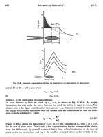
Figure 7. Classification of electric motors (42).
Other inertial type actuators are available which use,
for example, the piezoelectric effect, instead of a coil, to
move the inertial mass. Proof-mass actuators (also called
inertial actuators) are very similar in their operation to
electrodynamic shakers. They usually consist of a mass
that is moved by an alternating electromagnetic field.
These devices can generate relatively large forces and
displacements and can be good alternatives to costly
electrodynamic shakers. The devices can excite very stiff
structures such as electrical power transformers. Another
advantage of proof-mass actuators is that their resonant
frequency can be easily tuned for optimal efficiency at a
given frequency.
Electrical Motors
The advent of new control strategies and digital controllers
has revolutionized the way electrical motors can be used
and now allows for the use of motor technologies that were
previously difficult to implement in practical applications.
Simple motor drives were traditionally designed with
relatively inexpensive analog components that suffer from
susceptibility to temperature variations and component
aging. New digital control strategies now allow for the use
of electrical motors in active vibration control applications.
These efficient controls make it possible to reduce torque
ripples and harmonics and to improve dynamic behavior

in all speed ranges. The motor design is optimized due to
lower vibrations and lower power losses such as harmonic
losses in the rotor. Smooth waveforms allow an optimiza-
tion of power elements and input filters. Overall, these im-
provements result in a reduction of system cost and better
reliability.
Electrical motors can be divided into motors with a per-
manent magnet rotor (ac and dc motors) and motors with a
coiled rotor. Figure 7 illustrates a detailed classification of
the electrical motors. With the advent of new controllers,
the tendency is to classify electrical motors under ac or dc
according to the control strategy.
Due to its high reliability and high efficiency in a re-
duced volume, the brushless motor is actually the most
P1: FCH/FYX P2: FCH/FYX QC: FCH/UKS T1: FCH
PB091-V-Drv January 10, 2002 21:38
VIBRATION CONTROL IN SHIP STRUCTURES 1107
interesting motor for application to active vibration control
(40). Although the brushless characteristic can be applied
to several kinds of motors, the brushless dc motor is con-
ventionally defined as a permanent magnet synchronous
motor with a trapezoidal back EMF waveform shape, while
the brushless ac motor is conventionally defined as a per-
manent magnet synchronous motor with a sinusoidal back
EMF waveform shape. New brushless and coreless motors
are now available which are very linear over a wide speed
range (41). The brushless motor control consists of generat-
ing variable currents in the motor phases. The regulation
of the current to a fixed 60
◦

reference can be realized in two
modes: pulse width modulation (PWM) or hysteresis mode.
Shaft position sensors (incremental, Hall effect, resolvers)
and current sensors are used for the control. Linear per-
manent magnet motors are also available that, in addition
to the linear action, allow better magnetic dissipation in
the core as it is distributed in space.
If volume is not a major concern, a second type of motor
to be used in active vibration control is the induction or
ac motor (41). As for the brushless motor, the performance
of an ac motor is strongly dependent on its control. DSP
controllers enable enhanced real time algorithms. There
are several ways to control an induction motor in torque,
speed, or position; they can be categorized in two groups:
the scalar and the vector control. Scalar control means that
variables are controlled only in magnitude, and the feed-
back and command signals are proportional to dc quanti-
ties. The vector control is referring to both the magnitude
and phase of these variables. Pulse width modulation tech-
niques are also used for the control of inductionmotors, and
indirect current measurement (using a shunt or Hall effect
sensor) is used as a feedback information for the controller.
The third electrical motor used for active vibration con-
trol is the switched reluctance motor (40). This motor is
widely used mainly because of its simple mechanical con-
struction and associated low cost and secondarily because
of its efficiency, its torque/speed characteristic and its very
low requirement for maintenance. This type of motor, how-
ever, requires a more complicated control strategy. The
switched reluctance motor is a motor with salient poles on

both the stator and the rotor. Only the stator carries wind-
ings. One stator phase consists of two series-connected
windings on diametrically opposite poles. Torque is pro-
duced by the tendency of its movable part to move to a
position where the inductance of the excited winding is
maximized. There are two ways to control the switched re-
luctance motor in torque, speed and position. Torque can
be controlled by the current control method or the torque
control method. The pulse width modulation (PWM) strat-
egy is used in both current and torque control approaches
to drive each phase of the switched reluctance motor ac-
cording to the controller signal.
Hydraulic and Pneumatic Actuators
Hydraulic and pneumatic actuators are good candidate
technologies when low frequency, large force, and displace-
ments are required. Hydraulic actuators consist of a hy-
draulic cylinder in which a piston is moved by the action
of a high-pressure fluid. The main advantage of hydraulic
actuators is their large force and large displacement capa-
bility for a relatively small size. The disadvantages include
the need for a hydraulic power supply (which can require
space and generate noise), the high cost of servo-valves,
the nonlinear relation between the servo-valve input volt-
age and the output force or displacement produced by the
actuator, and the limited bandwidth of the actuator (0–
150 Hz). Hydraulic actuators have been used in the design
of active dynamic absorbers for ship structures (42,43).
The principle of operationofpneumatic actuators is very
similar to hydraulic actuators, except that the hydraulic
fluid is replaced by compressed air. Due to the higher com-

pressibility of air, the bandwidth of pneumatic actuators
is reduced (typically 0–10 Hz), which restricts the applica-
tion to nonacoustic problems. Pneumatic actuators may be
an attractive option when an existing air supply is already
available
APPLICATIONS OF NOISE CONTROL
IN SHIP STRUCTURES
A typical marine diesel engine mounted on a ship hull
is schematically depicted in Fig. 1. The figure shows the
various vibroacoustic paths through which the engine vi-
bration is transmitted to the ship structure, and eventu-
ally radiated into seawater. In the figure the coupling be-
tween structural and acoustic energy is classified using the
following symbols: AA: acoustic to acoustic coupling, SS:
structural to structural coupling, AS: acoustic to structural
coupling, SA: structural to acoustic coupling. The relative
importance of energy coupling for radiation into seawater
is illustrated by a number. As shown, there are five possi-
ble energy transmission paths, including (1) the mounting
system, consisting of the engine cradle, isolation mounts,
raft, and foundation; (2) the exhaust stack; (3) the fuel in-
take and cooling system; (4) the drive shaft; and (5) the
airborne radiation of the engine. In this study, these five
paths are grouped into four categories, corresponding to
generic active control problems:
r
Path 1: Active vibration isolation (mounting system).
r
Path 2: Active control of noise in ducts and pipes (ex-
haust stack; fuel intake and cooling system).

r
Path 3: Active control of vibration propagation in
beam-type structures (drive shaft).
r
Path 4: Active control of enclosed sound fields (air-
borne radiation of the engine).
Path 1: Active Vibration Isolation
Active vibration isolation involves the use of an active sys-
tem to reduce the transmission of vibration from one body
or structure to another (e.g., transmission of periodic vi-
bration from a ship’s engine to the ship’s hull). Such an
active isolation system will be used in practice to comple-
ment passive, elastomeric isolation mounts between the
engine and supporting structure. An active isolation sys-
tem is usually much more complex and expensive than
its passive counterpart, but has the advantage of offer-
ing better low-frequency isolation performances, and can
P1: FCH/FYX P2: FCH/FYX QC: FCH/UKS T1: FCH
PB091-V-Drv January 10, 2002 21:38
1108 VIBRATION CONTROL IN SHIP STRUCTURES
be designed for a better static stability of the supported
equipment.
The first class of system involves the control of sys-
tem damping, and is often referred as a semiactive isola-
tion system, Fig. 8(a). The damping modification is usually
achieved by a hydraulic damper with varying orifice sizes.
This system is often used for active suspensions in cars.
Such a system involves control time constants significantly
longer than the disturbance time constants, with the ad-
vantage of a simpler and less expensive implementation.

However, low-frequency performance is much less than for
fully active systems described in the following.
A second class of system involves an active control ac-
tuator in parallel with a passive system, with the actuator
Vibrating body
Spring
(a)
Variable
damper
Vibrating body
Spring
(b)
Control actuator
Damper
Vibrating body
Spring
(c)
Control actuator
Damper
Intermediate
mass
Figure 8. Active vibration isolation systems: (a) semiactive sys-
tem with variable damper; (b) active system with control force ap-
plied to both vibrating body and base structure; (c) active system
with control force in series with passive mount.
exerting a force on either the base structure or the rigid
mass, Fig. 8(b). In this parallel configuration, the actua-
tor is not required to withstand the weight of the machine;
as compared to the configuration of Fig. 8(c), the required
control force is smaller above the natural frequency of the

system (44). The main disadvantage of this configuration
is that at higher frequency (outside the frequency range
where the actuator is effective), the actuator itself can be-
come a transmission path. At low frequency, the large dis-
placement/large force requirements for heavy structures
preclude the use of piezoelectric, magnetostrictive actua-
tors. Instead, hydraulic, pneumatic, or electromagnetic ac-
tuators (with their associated weight, space, and possibly
fluid supplies problems) must be used. As far as practical
application of active control is concerned, the use of an ac-
tuator in parallel with a passive isolation stage could have
distinct advantages. In a given application, if an actuator
can be found that provides a control force of the order of the
primary force exciting the machine, then it may be possible
to use of much higher mounted natural frequency associ-
ated with the passive isolation stage than would be other-
wise possible. This in turn has advantages for the stability
of the mounted machine.
A third configuration with the active system in series
with the passive mount is shown on Fig. 8(c). Such a sys-
tem has several advantagesoverthe parallel configuration.
The active system is now isolated from the dynamics of the
receiving structure, which simplifies the control in the case
of a flexible base structure, and the use of an intermediate
mass creates a two-stage isolation system that offers better
isolation performance in higher frequency.
Path 2: Active Control of Noise in Ducts and Pipes
The reduction of duct noise is the first-known application
of active noise control. Active control systems for duct noise
are now a mature technology, with several commercial sys-

tems available for ventilation systems, chimney stacks, or
exhausts. All existing commercial systems are based on
feedforward adaptive control systems. In the case of ducts
containing air or a gas, loudspeakers are generally used as
control sources, and microphones as error sensors.
Two important classes of systems must be distin-
guished, depending on the frequency and the cross-
sectional dimension of the duct:
1. Systems for which only plane wave propagation ex-
ists in the duct. Such systems will necessitate a
single-channel control system (one control source and
one error sensor).
2. Systems for which higher-order acoustic modes prop-
agate in the duct. Such systems will require a multi-
channel control system.
The occurrence of higher-order modes in a duct depends
on the value of the cut-on frequency. For a rectangular
duct, the cut-on frequency is given by f
c
= c
0
/2d, where d
is the largest cross-sectional dimension and c
0
is the speed
of sound in free space. For a circular duct, f
c
= 0.586 c
0
/d,

where d is the duct diameter.Higher-order modes will prop-
agate at frequencies larger than f
c
.
P1: FCH/FYX P2: FCH/FYX QC: FCH/UKS T1: FCH
PB091-V-Drv January 10, 2002 21:38
VIBRATION CONTROL IN SHIP STRUCTURES 1109
For active noise control (ANC) in the large duct, mul-
tichannel acoustical ANC systems are necessary, and M
error sensors have to be used to control M modes for high-
order propagation cases. The error sensors should not be
located at the nodal lines (observability condition) (45). For
a rectangular duct, the location of the error sensors is rel-
atively simple because the nodal lines are fixed along the
duct axis. However, in circular ducts, the location of the
nodal lines changes along the duct axis, since the modes
usually spin as a function of the frequency, temperature,
and speed (46,47). Those variations of the nodal lines may
explain why ANC of high-order modes in circular or ir-
regular ducts appears to be difficult (48). Instead of using
the modal approach (i.e., the shape of the modes to be con-
trolled) to determine the error sensors location, an alterna-
tive strategy has recently been proposed by A. L’Esp
´
erance
(49)—the error sensor plane concept. This concept calls
for a quiet cross section to be created in the duct so that,
based on the Huygen’s principle, the noise from the pri-
mary source cannot propagate over this cross section. A
multichannel ANC in a circular duct accords with this

strategy (50).
The principles of active control of noise propagating in
liquid-filled ducts are much the same as in air ducts (51).
The higher speeds of sound in liquids means that plane
wave propagation occurs in a larger frequency range than
in air ducts. However, considerable care must be exercised
to the possible transmission of energy via the flexible duct
walls in this case, as a result of the strong coupling between
the duct walls and the interior fluid.
Path 3: Active Control of Vibration Propagation
in Beam-Type Structures
The active control of vibration in one-dimensional systems
such as beams, rods, struts, and shafts can be approached
from two different perspectives, depending on the descrip-
tion of the structural response. The response can be de-
scribed in terms of vibration modes or in terms of waves
propagating in the structure. The modal perspective is
more appropriate to finite, or short, beams and to global
reduction of the vibration. The description of the response
in terms of structural waves is more appropriate to infi-
nite, or long, beams and to reducing energy flow from one
part of the beam to another (control of vibration trans-
mission). The wave description is then more appropriate
to the case of the transmission of vibration from a ship’s
engine via the drive shaft, since in this case the source
of vibration is known and the objective is to block the vi-
bration transmission along the shaft. The active control
of vibration in beams is widely covered in the literature
(21,44). The following presentation is mostly limited to
feedforward control systems, since it is assumed that for

the problem of vibration transmission along a marine drive
shaft, an advanced signal correlated to the disturbance,
or a measurement of the incoming disturbance, wave is
possible.
Simultaneous Control of All Wave Types (Flexural,
Longitudinal, Torsional). In a general adaptive feedforward
controller used for the active control of multiple wave types
in a beam, sensor arrays (e.g., accelerometer arrays) are
used to measure the different types of waves propagating
upstream (detection array) or downstream (error array) of
the control actuators, and an array of actuators is used to
inject and control the various wave types in the beam (44).
Wave analyzers are necessary to extract the indepen-
dent wave types (assumed uncoupled) from the sensor ar-
rays, and wave synthesisers are necessary to generate the
appropriate commands to the individual actuators. This
approach has the advantage that independent control fil-
ters can be used to control the flexural, longitudinal, and
torsional waves. However, it necessitates excellent phase
matching of the sensors and a detailed knowledge of the
structure in which the waves propagate. An experimen-
tal laboratory implementation of this approach has been
conducted by (52), on a thin beam, for the control of two
flexural wave components and one longitudinal wave using
PZT actuators. Another, easier option avoids implementing
wave analyzers and synthesisers by simply minimizing the
sum of squared output of the error sensors to control the
different wave types. This approach, however, requires a
fully coupled multichannel control system. This approach
has been tested for the control of two flexural waves and

one longitudinal wave in a strut using three magnetostric-
tive actuators (53,54).
Control of Flexural Waves. The dispersive nature of flex-
ural waves implies that a control force applied transversely
to the beam generatespropagativewaves as wellasevanes-
cent waves localized close to the point of application of the
force. If one transverse control force is applied at some
location on the beam, it generates downstream and up-
stream propagating waves plus downstream and upstream
evanescent waves. This actuator can minimize the total,
transmitted downstream wave, but it generates a reflected
wave toward the source and two evanescent components
that may be undesirable. A total of four actuators will be
necessary to control downstream and upstream, propagat-
ing, and evanescent components. Therefore, the control of
flexural waves in beams will in general require actuator
arrays (55). Combinations of force and moment actuators
can also be used in the actuator array. The simplest feedfor-
ward control system uses only one control force and one er-
ror accelerometer, together with one reference accelerom-
eter to measure the incoming wave. This system has been
studied theoretically (56), and tested experimentally (57).
Physical limits of this system have been identified. The
first limit is associated with the detection of the control
actuator evanescent wave by the error sensor that puts a
limit on the actuator-error sensor separation: in practice,
the sensor should be at least 0.7 from the control actua-
tor (λ being the flexural wavelength). The second limit is
related to the delay between detection and actuation that
should be sufficient to allow the active control system to

react at the control actuator location before the primary
wave has propagated from the detection sensor to the con-
trol actuator. This puts a limit on the reference sensor–
actuator separation, which depends on the characteristics
of the control system.
Similarly to control actuator arrays, error sensor arrays
need to be implemented for the control of flexural waves
P1: FCH/FYX P2: FCH/FYX QC: FCH/UKS T1: FCH
PB091-V-Drv January 10, 2002 21:38
1110 VIBRATION CONTROL IN SHIP STRUCTURES
Disturbance
shaker
0
L
x
Accelerometer probe
error sensor
Laser
vibrometer
Piezoelectric
patch control
actuator
Figure 9. Typical experimental setup for the control of active
structural intensity.
to distinguish between the various propagating waves and
evanescent waves at the error sensor locations. This is par-
ticularly needed if the error sensors must be located at
a short distance from the control actuators. In this case,
an array of four accelerometers can discriminate between
the two propagating waves and the two evanescent waves

at the location of the error sensor array, and extract the
components that need to be reduced (e.g., the downstream
propagating wave).
Other sensing strategies have also been suggested, such
as measuring and minimizing the structural intensity due
to flexural waves (58,59). Structural intensity can be mea-
sured in practice using an array of four or more closely
spaced accelerometers, as presented in Fig. 9.
Practical Implementations. There are a limited number
of practical implementations of these principles to large,
machinery structures. Semiactive or active devices have
been used to attenuate the transmission of longitudinal
vibration on a large tie-rod structure (60). The tie-rod is
similar to that found in marine machinery to maintain the
alignment of a machinery raft. A tunable pneumatic vi-
bration absorber was used as the semiactive device, and
an electrodynamic shaker or a magnetostrictive actuator
was used as the active device. A load cell was used as the
error sensor, such that the force applied by the tie-rod to a
receiving bulkhead was minimized.
The suppression of vibration that is generated on ro-
tating machinery with an overhung rotor has been pre-
sented (61). In this case, the vibration of the rotor-shaft
system is controlled by active bearings. The active bear-
ings consist of a bearing housing supported elastically by
rubber springs and controlled actively by electromagnetic
actuators. These actuators are controlled by displacement
sensors at the pedestal and/or the roller and can apply an
electromagnetic force that suppresses any vibration of the
roller. The active vibration control (AVC) of rotating ma-

chinery utilizing piezoelectric actuators was also investi-
gated (62). The AVC is shown to significantly suppress vi-
bration through two critical speeds of the shaft line.
Path 4: Active Control of Enclosed Sound Fields
There exists a vastbody of literature on the subjectof active
control of enclosed sound fields. Only the previous work re-
levant to the problem of canceling the sound field radiated
by a ship engine in its enclosed space will be reviewed here.
More comprehensive presentations of the generic problem
can be found in (3,21). Active control of enclosed sound
fields has found applications essentially for automobile in-
terior noise (63,64) and for aircraft interior noise (65–67),
leading in some cases to commercial products.
There are two main categories of active control systems
related to enclosed sound field minimization:
r
Active control of sound transmission through elastic
structures into an enclosure.
r
Active control of sound field into rigid enclosures.
Only the second category will be reviewed here. The active
control of sound transmission has been investigated using
essentially modal approaches (68,69). The same type of an-
alytical approach based on modes of the acoustic enclosure
can be used to investigate the active control of sound field
into rigid enclosures. It should be mentioned, however, that
finite element approaches have also been used to study
the active control of sound field into enclosures of com-
plex geometries (70,71). Additionally, the objective of the
active control in an enclosure can be to minimize the sound

field globally,orlocally. Only the approaches directed to-
ward global attenuation of the sound field are reviewed
here. In this respect, some important physical aspects of
this problem are discussed in the following. These physi-
cal aspects depend primarily on the modal density of the
enclosure.
Enclosures with a Low Modal Density. For enclosureswith
a low modal density (i.e., a small enclosure, or at low fre-
quency), the active control will usually consist of placing
a series of control loudspeakers in the enclosure; the loud-
speakers are driven to minimize the sound pressure mea-
sured by discrete error microphones. In the case of an
enclosed acoustic space, the performance metrics for the
control should be the acoustic potential energy integrated
over the volume of the enclosure,
E
p
=
1
4ρ
0
c
0
2

V
|p(r)|
2
dv,
where p(r) is the local sound pressure, ρ

0
is the density
of the acoustic medium, and c
0
is the speed of sound. The
active control scheme should aim at reducing the acoustic
potential energy as much as possible.
It has been shown that active control of sound fields
in lightly damped enclosures is most effective at the res-
onance of the acoustic modes (72). In these instances, the
problem is essentially the control of a single mode. Sig-
nificant attenuation of the acoustic potential energy is
obtained using a single control source and a single er-
ror microphone (provided that neither the control source
nor the error microphone is located on a nodal surface of
the acoustic mode). For a multiple-mode (off-resonance)
response of the cavity, the number of control sources
and error microphones should be increased. However, the
potential for attenuation is never as large as at a resonance
frequency.
P1: FCH/FYX P2: FCH/FYX QC: FCH/UKS T1: FCH
PB091-V-Drv January 10, 2002 21:38
VIBRATION CONTROL IN SHIP STRUCTURES 1111
The number and placement of control sources and error
sensors are critical for multiple-mode control. The corre-
sponding optimization problem is nonlinear and usually
involves many local minima. Optimization processes, such
as multiple regression (21) or genetic algorithms (73), are
used. As a general rule is that the number and locations
of the control sources should be such that the secondary

sound field matches as closely as possible the primary
sound field in the enclosure.
Enclosures with a High Modal Density. As the frequency
increases or the enclosure becomes larger, global attenua-
tion of the sound field becomes more difficult to achieve us-
ing an active control system. To quantify these limitations,
there are some approximate formulas, which are summa-
rized here. These formulas are approximate, but they give
useful expected performance of an active control system in
a high modal density enclosure.
First, assuming a single primary point source and a sin-
gle secondary point source in the enclosure, it is possible
to derive the ratio of the minimized potential energy (after
control) to the original potential energy (before control),
(74):
E
p,min
E
p,0
= 1 −

1 +
π
2
M(ω)

−2
,
where M(ω) is the modal overlap of the cavity, which
quantifies the likely number of resonance frequencies of

other modes lying within the 3 dB bandwidth of a given
modal resonance. For a rigid rectangular enclosure and for
oblique acoustic modes, namely three-dimensional modes,
such as the (1,1,1) mode,
M(ω) =
ζω
3
V
πc
0
3
,
where ζ is the damping ratio in the enclosure (assumed
identical for all acoustic modes), ω is the angular frequency
of the sound field, and V is volume of the enclosure.
If the modal density is low (at low frequency),
E
p,min
E
p,0
≈ π M(ω ),
which means that the achievable attenuation is dictated
by the modal overlap (and hence the modal density and
damping of the enclosure).
If the modal density is large (at high frequency),
E
p,min
E
p,0
≈ 1,

which means that no attenuation can be obtained
after control. Another expression can be derived from
the asymptotic expression of modal overlap in high
frequency (75),
E
p,min
E
p,0
= 1 −sin c
2
kd,
where k is the acoustic wave number and d is the separa-
tion between the primary and control sources. Thus, as the
control source becomes remote from the primary source,
such that kd ≥ π, any global attenuation of the sound field
becomes impossible. This provides an explicit analytical
demonstration that the global control of enclosed sound
fields of high modal density is only possible with closely
spaced compact noise sources. In other words, assuming an
extended primary source such as a ship engine, the only vi-
able solution in this case is to distribute control loudspeak-
ers around the engine and in the close vicinity of it (within
a fraction of the acoustic wavelength).
Advanced Sensing Strategies. Recently, alternatives to
sensing and minimizing squared sound pressure have been
suggested in active control of enclosed spaces. Sensing
strategies based on total acoustic energy density minimiza-
tion instead of soundpressure minimization have been sug-
gested (76,77). The advantage of sensing the total energy
density is that the control is less sensitive to the sensor lo-

cations, and in general, a superior attenuation is obtained.
The energy density can be measured using combinations of
microphones (2 to 6); in this case, finite differences between
individual microphones are applied to obtain approximate
measurements of the pressure gradient in several direc-
tions. Precise measurements of the pressure gradient re-
quires an excellent phase matching of the individual micro-
phones, which can result in more expensive microphones.
Associated adaptation algorithms for the minimization of
energy-based quantities have been derived (78).
RECOMMENDATIONS ON SENSORS AND ACTUATORS
FOR ANVC OF MARINE STRUCTURES
Steps in Design of Active Control Systems
in Marine Structures
The choice of the sensors and actuators in an active con-
trol system will depend on factors such as the frequency
of the disturbance, operating environment, cost, expected
performance, and magnitude of the vibratory or acoustic
disturbance to be controlled along the various vibroacous-
tic paths. Figure 10 suggests a systematic approach that
proceeds through the various steps of the active control
system design. As a general recommendation, the first (and
perhaps most important) phase of the design of every ac-
tive control system is to acquire a thorough understanding
of the vibroacoustic behavior of the system on which active
control is to be applied. This involves carefully identifying
and ranking the various paths along which vibroacoustic
energy flows. This may imply addressing questions such
as the transmission of moments or in-plane forces through
the engine mounting, or the relative contribution of fluid-

borne and structure-borne energy along pipes. This early
phase is crucial in determining the active control strategy
to be implemented. A number of experimental techniques
and numerical simulation tools can be used to estimate
the relative contribution of the various paths at a given
receiving point (e.g., in water). Based on some contractors’
previous experiences, a major transmission path appears
to be the engine-mounting system.
P1: FCH/FYX P2: FCH/FYX QC: FCH/UKS T1: FCH
PB091-V-Drv January 10, 2002 21:38
1112 VIBRATION CONTROL IN SHIP STRUCTURES
Phase 1– Understanding the vibroacoustics of the
system
Phase 2–Selecting the control actuators
Identifcation of the transmission paths
Ranking of the transmission paths
Active control strategy
•
•
•
Frequency of the disturbance
Magnitude of the disturbance
Mechanical impedance of the structure
•
•
Phase 3–Selecting the error sensors
Phase 4–Testing the active control system
Exact quadratic optimization
Error sensor configuration for
global control

•
•
•
Control paths transfer function
measurements
•
Figure 10. Suggested design steps of an active control system.
The second phase will determine the type, number, and
locations of the control actuators. When global control is
desirable (e.g., when attenuation of the sound field is de-
sired at all positions in water), these parameters are deter-
mined by the requirement that the sound field generated
by the control actuators should spatially match the pri-
mary sound field. The type of control actuators to be used
will be based primarily on the frequency of the disturbance
and the magnitude of the disturbance at the actuator loca-
tion (for simplicity, the control actuators need to generate a
secondary field with a magnitude equal to the disturbance
at the actuator location). Once the type, number, and loca-
tions of the control actuators are known, extensive transfer
function measurements need to be taken between individ-
ual actuators and field points (vibratory or acoustic), with
the primary source turned off. Since this may involve a con-
siderable experimental task, numerical simulations can be
of a great help here.
The third phase will address the error sensors. Again, if
global control is desirable, the type, number, and locations
of the error sensors are dictated by the requirement that
if the control actuators are driven to minimize the signal
at the error sensors, then the resulting sound field is glob-

ally reduced. The measured transfer functions between in-
dividual actuators at field points and the magnitude of
the primary disturbance at these field points are used,
in conjunction with classical exact quadratic optimization
techniques, to calculate the optimal control variables (i.e.,
the required inputs of the control actuators) that minimize
the error signals for a given error sensor arrangement. The
final phase will be to test the active control with a real
controller.
Recommended Sensor and Actuator Technologies
for Various Ship Noise Paths
Path 1: Active Vibration Isolation. In selecting sensors
and actuators for active vibration isolation of engine noise,
due consideration has to be given to the size and weight
of the structure (engine) being isolated. Since the engine
is a heavy structure weighing over 6000 kg, it is neces-
sary that that the actuators are capable of delivering very
high control forces. In addition, the nature of the noise
through this path is nonacoustic, and hence nonacoustic
sensors and actuators have to be used. Based on these con-
siderations, the recommended sensors and actuators are
(1) accelerometers and force transducers for sensing and
(2) hydraulic and electrodynamic actuators for actuation.
The recommendations are summarized in Table 3. For in-
creased efficiency, the control systems must be designed
to provide control forces in translational and rotational di-
rections, since engine vibrations could take place in all di-
rections. Furthermore, the active control systems should
be used in conjunction with passive control systems, to re-
duce cost as well to provide fail-safe designs.

Path 2: Active Control of Noise in Ducts and Pipes. The
feedforward algorithm has been recommended for the con-
trol of noise associated with a marine diesel engine where a
reference signal is accessible (4). For ducts, generally asso-
ciated with large cross-sectional dimensions, higher-order
modes are more likely to exist, requiring a large number
of sensors and actuators with an appropriate positioning
strategy. For pipes, generally associated with small cross-
sectional dimensions, it is expected that only plane wave
propagation will exist, thereby limiting the number of ele-
ments needed to one sensor andone actuator. The following
sensing configurations are possible: microphones, piezo-
electric sensors, or accelerometers. For actuation, loud-
speakers and inertial actuators are recommended.
Path 3: Active Control of Vibration Propagation in
Beam-Type Structures. Feedforward control was recom-
mended for the vibration control of a propeller shaft (4).
The configuration of sensors and actuators to be used will
depend on the excitation source and on the modal behavior
of the shaft. For modal control, the sensors and actuators
can be located either on the shaft itself or connected to
it by a stationary mechanical link, such as by a bearing
mounted on the shaft. Potential mounted actuators include
curved piezoelectric actuators (PZT) and magnetostric-
tive actuators. For wave transmission control, sensors and
actuators arrays are required to measure the downstream
propagating and evanescent waves and to inject the control
waves in the structure.
Mounted sensors to be used include piezoelectric
(PVDF) sensors to measure the strain and accelerometers,

P1: FCH/FYX P2: FCH/FYX QC: FCH/UKS T1: FCH
PB091-V-Drv January 10, 2002 21:38
VIBRATION CONTROL IN SHIP STRUCTURES 1113
Table 2. Properties of Selected Piezoelectric Materials
BM532 Motorola
Property PZT-4 PZT-5H Piezoceramic 3203 HD PZT PZT-G1195N
Elastic properties
E
11
(GPa) 81.3 170.0 71.4 1.77 63
E
22
(GPa) 81.3 170.0 71.4 1.77 63
E
33
(GPa) 64.5 158.0 5.0 1.77 63
G
12
(GPa) 30.6 23.0 27.5 0.681 24.2
G
23
(GPa) 25.6 23.0 27.5 0.681 24.2
G
13
(GPa) 25.6 23.0 27.5 0.681 24.2
<
12
0.33 0.3 0.3 0.3 0.3
<
13

0.3 0.3 0.3 0.3
<
23
0.3 0.3 0.3 0.3
Piezoelectric coefficients (10
12
m/V)
d
31
−122 −200 −295 −254
d
32
−122 −200 −295 −254
d
33
285 580 569 374
d
24
0 560 584
Piezoelectric stress constants (C/m
2
)
e
31
−6.5
e
32
−6.5
e
33

23.3
e
23
17.0
Electric permittivity
γ
11
/γ
0
1480 1695 3250 2418 1729
γ
22
/γ
0
1480 1695 3250 2418 1729
γ
33
/γ
0
1300 1695 3250 3333 1695
Mass density 7600 7500 7350 7600
 (kg/m
3
)
Note: γ
0
= 8.85 ×10
−12
farad/m, electric permittivity of air.
if the rotation speed permits, for acceleration measure-

ment. The mounted actuators include piezoelectric (PZT)
actuators to induce strain in the structure. For robust-
ness, it is recommended that the actuators be combined
with passive control elements such as a viscoelastic layer
bonded to the shaft.
Table 3. Recommended Sensors and Actuators for Ship Noise Control
Recommended Sensors and Actuators
Ship Noise Path Sensors Actuators
Path 1: Active vibration isolation
r
Force transducers
r
Hydraulic actuators
r
Accelerometers
r
Electrodynamic actuators
Path 2: Active control of noise
r
Microphones
r
Loudspeakers
in ducts and pipes
r
Piezoelectric sensors
r
Electric motors
r
Accelerometers
Path 3: Active control of vibration

r
Piezoelectric sensors
r
Piezoelectric actuators
propagation in beam-type structures
r
Accelerometers
r
Magnetostrictive actuators
r
Electrodynamic shakers
r
Electrodynamic shakers
r
LVDT
Path 4: Active control of airborne
engine noise
Sound field into enclosures
r
Combination microphones
r
Loudspeakers
r
Accelerometers
Radiated noise into sea
r
Piezoelectric sensors
r
Piezoelectric actuators
r

Accelerometers
r
Magnetostrictive actuators
Path 4: Active Control of Radiated Sound Fields. There
are two types of radiated noise to be controlled for ship
structures. These are the airborne engine noise into an en-
closure, and the noise radiated by the noise into the sea.
As stated in (4) both cases require the use of global con-
trol techniques that involve multiple input and multiple
P1: FCH/FYX P2: FCH/FYX QC: FCH/UKS T1: FCH
PB091-V-Drv January 10, 2002 21:38
1114 VIBRATION CONTROL IN SHIP STRUCTURES
output transducers. Control of radiated noise can be
achieved either by active noise cancellation (ANC) or by
active structural acoustic control (ASAC) techniques. For
active cancellation, the following sensors and actuators
are recommended: (1) combination microphones and ac-
celerators as sensors and (2) loudspeakers as actuators.
For active structural acoustic control the following sen-
sors and actuators are recommended: (1) piezoelectric sen-
sors (shaped or not) and accelerometers as sensors, and (2)
piezoelectric and magnetostrictive materials as actuators.
SUMMARY AND CONCLUSIONS
Among the wide range of sensor and actuator materials
that could be used for active noise and vibration control in
ship structures are piezoelectric and electrostrictive ma-
terials magnetostrictive materials, shape-memory alloys,
optical fibers, electrorheological and magnetoeheological
fluids, microphones, loudspeakers, electrodynamic actua-
tors, and hydraulic and pneumatic actuators. In making

the selection, due consideration must be given to factors
such as cost, frequency of the disturbance, operating (ma-
rine) environment, experience in other applications, ease
of implementation, and the expected performance. In gen-
eral, the following recommendations are made:
1. Nonacoustic sensors and actuators (e.g., accelero-
meters, force transducers, hydraulic actuators, piezo-
electric materials, and electrodynamic actuators) are
best for nonacoustic paths, namely for the engine-
mounting system, the drive shafts, and mechanical
couplings.
2. Acoustic sensors and actuators (e.g., microphones
and loudspeakers) are best for acoustic paths, namely
for the exhaust stacks and piping systems, and the
air-borne noise.
It was also recommended that the active control strategies
be combined with passive treatments whenever possible,
to increase the robustness of the control system and to pro-
vide a fail-safe design.
BIBLIOGRAPHY
1. C.R. Fuller and A.H. von Flotow. IEEE Cont. Sys. Mag. 15(6):
9–19 (1995).
2. R.R. Leitch. IEEE Proc. 134(6): 525–546 (1987).
3. P.A. Nelson and S.J. Elliott. Active Control of Sound. Academic
Press, San Deogo, CA, 1992.
4. U.O. Akpan, O. Beslin, D.P. Brennan, P. Masson, T.S. Koko,
S. Renault, and N. Sponagle. CanSmart-99, Workshop,
St Hubert, Quebec, 1999.
5. J.C. Simonich. J. Aircraft. 33(6): 1174–1180 (1996).
6. S.S. Rao and M. Sonar. Appl. Mech. Rev. 47(4): 113–123 (1994).

7. V. Giurgiutiu, C.A. Rogers, and Z. Chaudhry. J. Intell. Mater.
Sys. Struct. 7: 656–667 (1996).
8. L. Bowen, R. Gentilman, D. Fiore, H. Pham, W. Serwatke,
C. Near, and B. Pazol. Ferroelectr. 187: 109–120 (1996).
9. S. Sherrit, H.D. Wiederick, B.K. Mukherjee, and S.E. Prasad.
Ferroelectr. 132:61–68 (1992).
10. Thunder™. Actuators and Sensors, FACE International Cor-
poration Product Information. 1997.
11. E.F. Crawley and J. de Luis. AIAA J. 25(10): 1373–1385 (1987).
12. V.V. Varadan, Y H. Lim, and V.K. Varadan. Smart Mater.
Struct. 5: 685–694 (1996).
13. H.S. Tzou and R. Ye, J. Vib. Acous. 116: 489–495 (1994).
14. T.S. Koko, I.R. Orisamolu, M.J. Smith, and U.O. Akpan. SPIE
Conf. on Smart Structures and Materials, Vol. 3039, pp. 125–
134 (1997).
15. H. Sumali and H.H. Cudney. AIAA-94-1406-CP, pp. 1233–1241
(1994).
16. A. Grewal, D.G. Zimcik, and B. Leigh. CanSmart Workshop
on Smart Materials and Structures, CSA, St Hubert, Quebec,
Canada, 1998.
17. D.L. Sutliff, Z. Hu, F.G. Pla, and L.J. Heidelberg. Proc. 3rd
AIAA/CEAS Aeroacoustic Conf., Atlanta, GA, AIAA-97-1641,
1997.
24. C. Liang and C.A. Rogers. J. Intell. Mater. Sys. Struct. 1: 207–
234 (1990).
25. T.S. Koko, U.O. Akpan, L. Guertin, A. Berry, and P. Masson.
DREA Contractor Report, in review (1999).
26. K. Tanaka. Res. Mechanic 18: 251–263 (1986).
39. I.C. Shepherd, R.F. La Fontaine, and A. Cabelli. J. Sound Vib.,
130: 125–135 (1989).

40. Texas Instruments. />appnotes.htm (1999).
41. Micro Mo Electronics. />(1999).
42. W.J. Hsueh and Y.J. Lee. Trans. ASME 116(1): 43–48 (1994).
43. T. Kakinouchi, T. Asano, K. Tanida, and N. Takahashi. Naval
Eng. J. 104(3): 46–52 (1992).
44. C.R. Fuller, S.J. Elliott, and P.A. Nelson. Active Control of Vi-
bration. Academic Press, New York, 1996.
45. S. Douglas and J. Olkin. Proc. Recent Advances on Active Con-
trol, 1993.
46. C.L. Morfey. J. Sound Vib. 1:60–87 (1964).
47. A. Bihhadi and Y. Gervais. Acta-Acoustica 2: 343–357 (1994).
48. S. Laugesen. J. Sound Vib. 195(1): 33–56 (1996).
49. A. L’Esp
´
erance, M. Bouchard, B. Paillard, C. Guigou, and A.
Boudreau. Appl. Acous. 57: 357–374 (1999).
50. A. L’Esp
´
erance, M. Bouchard, and B. Paillard. Canadian Inst.
Mining, Light Metal Sec. Metall. Soc. 90(1012): 94–99 (1997).
51. W.G. Culbreth, E.W. Hendricks, and R.J. Hansen. J. Acous.
Soc. Am. 83: 1306–1310 (1988).
52. R.L. Clark, J. Pan, and C.H. Hansen. J. Vib. Acous. 92(2): 871–
876 (1992).
53. M.J. Brennan, S.J. Elliott, and R.J. Pinnington. In Proc. 1st Int.
Conf. on Motion and Vibration Control, 1992, pp. 605–609.
54. S.J. Elliott, T.J. Sutton, M.J. Brennan, and R.J. Pinnington. In
Proc. IUTAM Symp. on the Active Control of Vibration, 1994,
pp. 1–8.
55. R.B. Mace. J. Sound Vib. 114: 253–270 (1987).

56. X. Pan and C.H. Hansen. J. Sound Vib. 165: 497–510 (1993).
57. S.J. Elliott and L. Billet. J. Sound Vib. 163: 295–310 (1993).
58. A.E. Schwenk, S.D. Sommerfeldt, and S.I. Hayek. J. Acoust.
Soc. Am. 96(5): 2826–2835 (1994).
59. P. Audrain, P. Masson, and A. Berry. J. Acous. Soc. Am. (1999)
in press.
P1: FCH/FYX P2: FCH/FYX QC: FCH/UKS T1: FCH
PB091-V-Drv January 10, 2002 21:38
VIBRATIONAL ANALYSIS 1115
60. M.J. Brennan, M.J. Day, andR.J. Randall.J. Vib. Acous. 120(1):
1–12 (1998).
61. K. Kato, T. Fujii, K. Mizutani, Y. Kurita. Trans. Jpn. Soc. Mech.
Eng. C63 (609): (1997).
62. A.B. Palazzolo, S. Jagannathan, A.F. Kascak, T. Griffin, and
J. Giriunas. ASME Int. Gas Turbine and Aero-engine Cong-
ress and Exposition 1993, pp. 1–12.
63. R.J. Bernhard. In Proc. Active 95, 1995, pp. 21–32.
64. T.J. Sutton, S.J. Elliott, A.M. McDonald, and T.J. Saunders.
Noise Contr. Eng. J. 42: 137–147 (1994).
65. S.J. Elliott, P.A. Nelson, I.M. Stothers, and C.C. Boucher. J.
Sound Vib. 140: 219–238 (1990).
66. I.U. Borchers, U. Emborg, A. Sollo, E.H. Waterman, J. Paillard,
P.N. Larsen, G. Venet, P. Goransson, and V. Martin. In Proc.
4th NASA/SAE?DLR Aircraft Interior Noise Workshop 1992.
67. U. Emborg and C.F. Ross. In Proc. Recent Advances in Active
Control of Sound and Vibration. 1993, pp. 100–109.
68. C.R. Fuller. J. Sound Vib. 109: 141–156 (1986).
69. J. Pan, C.H. Hansen, and D.A. Bies. J. Acous. Soc. Am. 87:
2098–2108 (1990).
70. C.G. Mollo and R.J. Bernhard. J. Vib. Acous. 112: 230–236

(1990).
71. K.A. Cunefare and G.H. Koopmann. J. Acous. Soc. Am. 90:
365–373 (1991).
72. A.R.D. Curtis, P.A. Nelson, and S.J. Elliott. J. Acous. Soc. Am.
88: 2265–2268 (1990).
73. K.H. Baek and S.J. Elliott. J. Sound Vib. 186: 245–267 (1995)
74. S.J. Elliott. ISVR Memorandum 695 (1989).
75. P.A. Nelson, A.R.D. Curtis, S.J. Elliott, and A.J. Bullmore. J.
Sound Vib. 117:1–13 (1987).
76. S.D. Sommerfeldt, J. Parkins, and Y. Park. In Proc. Active 95,
1995, pp. 477–488.
77. B.S. Cazzolato. Thesis. Department of Mechanical Engineer-
ing, University of Adelaide, 1998.
78. S.D. Sommerfeldt and P.J. Nashif. J. Acous. Soc. Am. 96: 300–
306 (1994).
VIBRATIONAL ANALYSIS
DAVE S. STEINBERG
Westlake Village, CA
INTRODUCTION
Vibration is present almost everywhere we travel in mod-
ern society. Vibrationally induced failures are very com-
mon in products such as television sets and computers
that are shipped by trains and trucks. Vibrational failure
in a television set may be just an inconvenience. However,
vibrational failure in a large passenger airplane can lead to
many deaths. Methods of vibrational analysis are available
that are accurate and can reveal weak structural areas.
Steps can then be taken either to repair or replace critical
items. Vibrational analysis is a combination of science and
art. The science uses sophisticated computers extensively

to solve large complex problems. This method requires ex-
tensive training and often takes a long time to reach a
satisfactory solution. The art uses approximations, short
cuts, and test data to reduce the time needed to reach a
satisfactory solution. The approximations and short cuts
can sharply reduce the time required for a solution, but it
also reduces the accuracy of the analysis. Vibrational anal-
ysis can be used to make some materials work smarter
by making small changes in their physical properties.
These changes can often increase the fatigue life of criti-
cal structural members without a significant increase in
the size, weight, cost, or impact on production and delivery
schedules.
VIBRATIONAL REPRESENTATION
In a broad sense, vibration means an oscillating motion,
where something moves back and forth. If the motion re-
peats itself, it is called periodic. If continuous motion never
repeats itself, it is called random motion. Simple harmonic
motion is the simplest form of periodic motion, and it is
typically represented by a sine wave, as shown in Fig. 1.
The reciprocal of the period is known as the frequency, and
it is measured in cycles per second, or hertz (Hz). The maxi-
mum displacement is called the amplitude of the vibration.
DEGREES OF FREEDOM
A coordinate system is usually used to locate the positions
of various elements in a system. When only one element is
involved, it is restricted to moving along only one axis, and
only one dimension is required to locate the position of the
element at any instant, then it is called a single-degree-of-
freedom system. The same is true for a torsional system.

When one element isrestrictedto rotating about one axis so
that only one dimension is required to locate the position of
the element at any instant, it is a single-degree-of-freedom
system. Two degrees of freedom requires two coordinates
to locate the positions of the elements, and so on.
A single rigid body is usually considered to have six
degrees of freedom, translation along each of the three
orthogonal x, y, and z axes and rotation about each of the
same three axes. Real structures are usually considered to
have an infinite number of degrees of freedom.
VIBRATIONS OF SIMPLE STRUCTURES
The natural frequency (often called the resonant fre-
quency) of a simple single-degree-of-freedom system can
+ Displacement
− Displacement
Amplitude
Time
Period
Figure 1. Simple harmonic motion: a sine wave.
P1: FCH/FYX P2: FCH/FYX QC: FCH/UKS T1: FCH
PB091-V-Drv January 10, 2002 21:38
1116 VIBRATIONAL ANALYSIS
CK
Chassis or
PCB
M
Figure 2. Single-degree-of-freedom spring-mass system.
often be obtained from the strain energy and the kinetic
energy of the system. Consider the single spring and mass
system shown in Fig. 2. When there is no damping in the

system, then no energy is lost, and the strain energy must
be equal to the kinetic energy. This results in the natural
frequency equation (1),
f
n
=
1
2π

g
Y
st
(Hz), (1)
where
g = 9.80 m/s
2
(386 in/s
2
), the acceleration of gravity and
Y
st
in meters (inch) is the static displacement.
Sample Problem: Natural Frequency of a Simple Structure
When the static displacement of a structure Y
st
= 1.27 ×
10
−5
m (0.00050 in), its natural frequency is 140 Hz.
The natural frequency is important because it is often

considered the heart of a vibrating system. It influences
the number of fatigue cycles and the displacement, which
affect the fatigue life of a system. It also influences the
damping, which affects the dynamic acceleration Q level,
and the stress level, which also affects the fatigue life.
NATURAL FREQUENCIES OF UNIFORM
BEAM STRUCTURES
Natural frequencies of uniform beam structures can be de-
termined by equating the strain energy to the kinetic en-
ergy without damping. This method of analysis leads to
simple solutions and very little error because beam types
of structures normally have very little damping. The re-
sulting equations for natural frequency apply to uniform
beams that are forced to bend only in the vertical axis with-
out bending in the horizontal axis and without torsion or
twisting. The beam equation is (1)
f
n
=
a
2π

EIg
WL
3
(Hz), (2)
where
a = 3.52 for a cantilevered beam,
a = π
2

= 9.87 for a beam that is supported (hinged) at
each end,
a = 22.4 for a beam that is clamped (fixed) at both ends,
E in newtons (N) m
2
(lb/s in
2
) is the modulus of elasticity
for beam material,
I in m
4
(in
4
) is the area moment of inertia for a beam
cross section,
g = 9.80 m/s
2
(386 in/s
2
), the acceleration of gravity,
W in Ns (N) (lb) is the total weight of the beam, and
L in m (in.) is the length of the beam between supports.
A
b
h
A
L
(10.0 in.)
0.254 meters
Section

AA
(2.0 in.)
0.0508 meters
0.0254 meters
(1.0 in.)
Figure 3. Uniform beam simply supported at each end.
Sample Problem: Natural Frequency of a Simply Supported
Uniform Beam
For example, consider the simply supported (hinged) alu-
minum beam shown in Fig. 3, where E = 6.894 × 10
10
N/m
2
(10 ×10
6
lb/in
2
), L = 0.254 m (10.0 in), I = 6.937 ×
10
−8
m
4
(0.1667 in
4
), and W = 8.896 N (2.0 lb). The result-
ing natural frequency is 890 Hz.
NATURAL FREQUENCIES OF UNIFORM PLATES
AND CIRCUIT BOARDS
The natural frequencies of different types of flat, uniform
plates that have different types of supports can often be

obtained by using trigonometric or polynomial series (1).
Again, when damping is ignored, the strain energy can
be equated to the kinetic energy of the bending plate
to obtain the natural frequency. A printed circuit board
(PCB) that supports and electrically interconnects various
electronic components can be analyzed as a flat rectan-
gular plate, often simply supported (hinged) on all four
sides, that has a uniformly distributed load across its sur-
face. The natural frequency for this type of installation
is (2).
f
n
=
π
2

D
ρ

1/2

m
2
a
2
+
n
2
b
2


(Hz), (3)
where
E in newtons/m
2
(lbs/in
2
) is the modulus of elasticity for
plate material,
h in m (in) is the plate thickness,
µ is Poisson’s ratio, dimensionless,
D =
Eh
3
12

1 −µ
2

N m (lb in), the plate bending stiffness
factor, (4)
ρ =
W
gab
Ns
2
/m
3
(lb s
2

/in
3
), the mass per unit area, (5)
g = 9.80 m/s
2
(386 in/s
2
), the acceleration of gravity,
W in newtons (lb), is the total weight of the PCB,
a in m (in) is the length of the plate,
b in m (in) is the width of the plate, and
m and n are integers: first harmonic m = 1, n = 1;
second harmonic m = 2, n = 1;
third harmonic m = 1, n = 2; fourth harmonic m = 2,
n = 2.
P1: FCH/FYX P2: FCH/FYX QC: FCH/UKS T1: FCH
PB091-V-Drv January 10, 2002 21:38
VIBRATIONAL ANALYSIS 1117
Y
X
X
b
a
Supported
Supported
Supported
Supported
h
Z
Z

0
Figure 4. Uniform flat plate simply supported on four sides.
Sample Problem: Natural Frequency of a Rectangular PCB
(see Fig. 4).
Consider a flat rectangular epoxy fiberglass PCB, sup-
ported (hinged) on four sides, where E = 1.379 × 10
10
N/s
m
2
, (2.0×10
6
lb/in
2
), h = 0.00157 m (0.062 in), µ = 0.12 di-
mensionless, D = 4.53 N (40.1 lb in), W = 4.448 N (1.0 lb),
a = 0.203 m (8.0 in), b = 0.178 m (7.0 in), ρ = 12.56 Ns
2
/m
3
(0.463×10
−4
lb s
2
/in
3
). The resulting natural frequency for
the first harmonic (m = 1, n = 1) is 52.6 Hz.
METHODS OF VIBRATIONAL ANALYSIS
Hand calculations are still being used extensively for sim-

ple sinusoidal and random vibrational analyses in small
companies due to the high costs of the computers, the spe-
cialized computer software, and the skilled personnel to
operate the computers. Many reference books are available
that show how to perform simplified vibrational analyses
on different types of simple structures. However, when
large complex structures are involved, hand calculations
are not adequatetoensure reasonable accuracy. Small com-
panies often subcontract the work to outside consulting
organizations that specialize in these areas. Sometimes it
can be cheaper, faster, and more accurate to build a model
of the structure, so it can be examined in a vibrational test
laboratory.
Most large companies rely extensively on various types
of computers and specially formulated finite element mod-
eling (FEM) software programs for vibrational analyses.
Their computers are usually networked together, so each
has access to the wide variety of software analytical pro-
grams available on the network. The new desktop personal
computers (PC) are very popular for vibrational analyses
using FEM. They are more powerful and faster than the
large main frame computers of a few years ago.
PROBLEMS OF VIBRATIONAL ANALYSIS
Almost all computers and computer software FEM pro-
grams for vibrational analysis agree within about 2% when
they are used to determine eigenvalues (resonant frequen-
cies) and eigenvectors (mode shapes) for many types of
complex structures. However, sample problems solved by
using different FEM software programs have shown sig-
nificant variations in their stress values. The stress val-

ues from four different FEM programs had a total varia-
tion of about 60%. This was 30% above the average stress
value of the four programs and 30% below the average
value for similar models of the same structure, subjected to
the same type of vibrational excitation. Different computer
FEM programs typically use different algorithms to define
the building blocks for their various beam, plate, and brick
elements. These algorithmic variations probably cause the
variations in the stress values. Because the fatigue life of
a structure is closely related to its stress value, significant
variations in the calculated stress levels can result in dra-
matic changes in the calculated fatigue life of a structure.
For example, the results of this investigation showed that
the fatigue life at the critical point in the structure can be
expected to vary across a wide range because of the vari-
ations in the calculated stress values. The fatigue life in
the lead wires of PCB electronic component parts can be
as much as five times greater than the average calculated
fatigue life, or it can be as little as one-fifth of the average
calculated fatigue life. [See Ref. 5, Chap. 12, Figs. 12.1–
12.19 for more detailed information on finite element
modeling.]
The results shown before may vary substantially. Only
four different FEM software programs were involved in
this investigation. At least several dozen new software
programs are available now. When the different modeling
techniques of different computer analysts are considered,
these factors are expected to have a significant impact on
the computer calculated stress values and the resulting
calculated fatigue life.

PROBLEMS OF MATERIAL PROPERTIES
Material properties are often difficult to evaluate for vi-
brational environments. The life of any structure excited
by vibration depends on the fatigue properties of the most
critical materials used in fabricating and assembling the
structure. When structural elementsareforced to bend and
twist back and forth, perhaps millions of times in severe
vibrational environments, three very important factors
have to be defined:
1. the very basic fatigue properties ofthematerials used
in the structure
2. The manufacturing tolerances that will affect the
physical dimensions of the parts
3. stress concentrations due to holes, notches, small
radii, and rapid sectional changes.
First, consider the basic fatigue properties of the mate-
rials in the structure. Test data have shown that there are
significant variations in the fatigue life of virtually identi-
cal parts that are machined to very close tolerances from
the same forging, as shown in Fig. 5. These test data are
plotted on log–log curves of stress (S) against the num-
ber of cycles (N ) to failure. Only one average straight-line
P1: FCH/FYX P2: FCH/FYX QC: FCH/UKS T1: FCH
PB091-V-Drv January 10, 2002 21:38
1118 VIBRATIONAL ANALYSIS
1
2
N
cycles to fail
N

1
S
b
1
=
N
2
S
b
2
Stress
S
Figure 5. S–N fatigue curve showing large variations in the life
test data.
usually represents the fatigue life properties of a material
(1,3–5). When all of the failure test data points for all of
the test samples are plotted, a wide variation in the fa-
tigue life is revealed. Because these are log–log plots, the
spread in the possible variation in fatigue life of virtually
identical parts can be very great, sometimes reaching val-
ues of 10 to 1. Engineers involved in vibrational and fa-
tigue life analysis do not like to reveal this type of data to
upper management personnel. Personal experience with
nontechnical upper management people is that they often
expect mechanical designers and analysts to predict the fa-
tigue life of their structures to within plus and minus 20%.
This is an almost impossible task, when all of the possible
variations are considered.
To compensate for these large variations in fatigue life
of virtually identical structural elements, safety factors

(sometimes called factors of ignorance) must be used when
these structures are being designed and analyzed. Build-
ing models for vibrational life testing in a laboratory can
be a great help in estimating the fatigue life of a structure.
However, if no tests are run or if the number of samples
tested is low, there is always the danger of erratic bursts
of high failure rates in the production units because of the
large scatter associated with fatigue.
Next, consider the effects of manufacturing tolerances
on the physical dimensions of the structural elements in an
assembly. Mass-produced products always show some vari-
ations in the physicaldimensions of what appear to beiden-
tical parts. Even die cast parts thataremade from the same
mold have slightly different physical dimensions. Some
manufactured devices, like the automatic transmission in
an automobile, can have many precision gears, ground to
very close tolerances. Holding very tight manufacturing
tolerances can be very expensive. Therefore, looser toler-
ances are used in production parts that do not require tight
tolerances for precision assembly work because they this
reduce costs. When manufactured parts that have loose tol-
erances are exposed to severe vibration, the failure rates
often go up and down erratically. Changes in the physical
dimensions of load-carrying structural members can alter
the load path through the structure, which can change the
dynamic loads and stresses in it. It is too expensive to keep
track of manufactured parts that have extremes in their
dimensional tolerances. These parts can be anywhere in
large production programs. This means that failures which
are difficult to predict and to control, may occur randomly

in harsh environments.
To reduce costs, for example, the electronics industry
tends to use very loose tolerances in the dimensions that
control the external physical sizes of the length, width, and
thickness of their printed circuit boards (PCBs) and elec-
tronic component parts. These large variations in tolerance
of these parts further increase the difficulty in trying to
predict the fatigue life accurately of electronic assemblies
that are exposed to different vibrational environments.
RELATION OF DISPLACEMENT TO ACCELERATION
AND FREQUENCY
Vibrational displacements are often very small, so they
are difficult to observe during vibrational tests. Because
these displacements are small, it does not mean that the
resulting stresses arealsosmall. Vibrational environments
usually impose alternating displacements and alternat-
ing stresses on various structural load-carrying elements
within a system. If the vibrating system experiences many
thousands of stress reversals, fatigue failures can occur
in critical structural members, even at relatively low dis-
placements and stress levels. This is the nature of fatigue
failures that occur at relatively low stress levels near small
holes, small notches, and sharp bends. These geometric
shapes are known as stress concentration factors, which
can increase peak stress levels in these areas by a factor of
3 or 4 or more (4).
When vibrational tests are run in a laboratory, the nor-
mal procedure is to use small accelerometers to monitor
the resulting acceleration values in different parts of the
structure. When an electrodynamic shaker is used to gen-

erate a sinusoidal wave for the vibrational test, the elec-
tronic control system will show the frequency of the im-
posed wave in cycles per second, or hertz (Hz). With this
type of setup, the test engineer will know the acceleration
level and the frequency at any instant. This information
is often incomplete without the resulting displacement at
any instant. The resulting displacement at any instant can
be obtained by considering a rotating vector that generates
a sinusoidal wave based on the full relationship (1),
Y = Y
0
sin t, (6)
where
Y is the displacement at any time,
Y
0
is the maximum single amplitude displacement from
zero to peak, and
 = 2π( f ) rad/s, the frequency.
The acceleration a can be obtained from the second
derivative of the displacement with respect to time from
the preceding equation. The maximum acceleration occurs
when the sine function is one. It is convenient to represent
P1: FCH/FYX P2: FCH/FYX QC: FCH/UKS T1: FCH
PB091-V-Drv January 10, 2002 21:38
VIBRATIONAL ANALYSIS 1119
the acceleration in terms of gravity units G:
G =
a
g

(gravity units, dimensionless), (7)
where
a in m/s
2
(in/s
2
) is the acceleration level and
g = 9.80 m/s
2
(386 in/s
2
), the acceleration of gravity.
The final results show the displacement Y
0
in terms of
the frequency f in Hz and the number of dimensionless
gravity units G :
Y
0
=
AG
f
2
(single amplitude displacement), (8)
where
A = 0.248 for meters displacement (9.8 for inch dis-
placement)
G is the acceleration, in gravity units, dimensionless
(same in English units), and
f is the frequency in cycles/s (Hz) (same in English

units).
Sample Problem: Finding the Displacement
from the Frequency and the G Level
For example, when the acceleration G level is 3.0 dimen-
sionless gravity units and the frequency is 120 Hz, the sin-
gle amplitude displacement is 0.0000517 m (0.00204 in).
This equation is probably the most important relation-
ship in the entire field of dynamics. It shows that when
any two of the parameters of Y
0
, G or f , are known, then
the third parameter is automatically known. This equation
can be used for sine vibration, random vibration, shock,
and acoustics (1).
EFFECTS OF VIBRATION ON STRUCTURES
Vibrational environments can dramatically magnify the
dynamic forces and stresses in differenttypesof structures,
when the structural natural frequencies are excited. Forces
and stresses can be magnified and amplified by factors of
10, 30, and even 100 in many different types of structures
for different types of vibrational excitation. The magnitude
of the magnification, called the transmissibility Q, often
depends on the amount of damping in the vibrating system.
Figure 6showsdamping for a single-degree-of-freedom sys-
tem. There are very few single-degree-of-freedom systems
in the real world. For example, consider a two-degree-of-
freedom system for an electronic assembly where the chas-
sis is mass1. The plug-in PCBs are attached to the chassis
so they are mass 2. The response of mass 1 will be the input
to mass 2. Testing experience, including different damping

methods, has shown that the transmissibility Q of PCBs as
mass 2 will depend far more on the dynamic coupling phase
relation and frequency ratio between mass 1 and mass 2
than the damping in either mass 1 or mass 2 because the
transmissibility Q’s between masses 1 and 2 do not add,
they multiply.
0
0.1
0.2
0.4
0.6
0.8
1.0
2
4
6
8
10
0.5 1.0 1.5 2.0
0
0.10
0.20
0.50
0.50
R
c
= 1.0
R
c
= 0

0.20
0.10
2.5 3.0
R
Ω
= =
Forcing frequency
Natural frequency
f
f
n
Q
=
Maximum output force
Maximum input force
Figure 6. Effects of damping on the transmissibility Q plots.
The Q of a system is defined as the ratio of the out-
put (or response of the system) divided by the input. The
output and the input are usually defined in terms of the
displacements, or the acceleration values. If the damp-
ing in a simple system is zero, the vibration theory states
that the value of the transmissibility Q will be infinite.
If the transmissibility Q is infinite, the resulting dynamic
forces and stresses will also be infinite. However, because
all real systems have some damping, Q can never be infi-
nite. However, in lightly damped systems, Q can be very
high. A high Q willresult in high forces, displacements,and
stresses, which can sharply reduce the fatigue life of the
structure.
ESTIMATING THE TRANSMISSIBILITY

Q IN DIFFERENT STRUCTURES
The transmissibility Q is strongly influenced by the damp-
ing in a vibrating structure. One form of damping is the
conversion of kinetic energy into heat. This can be shown
by rapidly bending a metal paper clip back and forth about
20 times through a large angle. Immediately place your fin-
ger on the paper clip in the bending area. This area will be
quite warm. It may even be hot. The strain energy of bend-
ing has been converted into heat energy, which cannot be
converted back into strain energy. It is lost energy. When
heat energy is lost,itmeans there is also a loss ofkineticen-
ergy. Therefore,when damping is increased in a vibrating
system, there is less energyavailable to convert into kinetic
energy. Less kinetic energy means that there is less energy
available to excite the structure at its natural frequency, so
that the transmissibility Q is decreased. Conversely, when
there is a decrease in the damping, this makes more kinetic
energy available to excite the structure, so the transmissi-
bility Q is increased.
P1: FCH/FYX P2: FCH/FYX QC: FCH/UKS T1: FCH
PB091-V-Drv January 10, 2002 21:38
1120 VIBRATIONAL ANALYSIS
In general, simple systems that have only a few struc-
tural elements have less damping than more complex sys-
tems that have many structural elements, when both sys-
tems are subjected to the same vibrational environment.
Bolted joints usually have a lot of friction and damping at
the bolted interfaces in vibrational environments, so struc-
tures that have many bolted joints usuallyhave high damp-
ing. Therefore, a simple beam type of structure usually has

less damping than a more complex plate type structure.
Then, a beam structure should have a higher transmis-
sibility Q than a plate structure in the same vibrational
environment. The same thinking can be applied to a more
complex box type of structure that has removable bolted
covers to provide access to internal subassemblies. The box
type of structure should have more damping than the plate
structure for similar vibrational exposure because the box
structure is much more complex than a plate structure.
This means that the box structure should have a lower
transmissibility Q than the plate structure for similar vi-
brational exposure. Extensive vibrational test data shows
that this is the natural trend for damping in different types
of structures.
Higher dynamic forces in a structure typically result
in higher dynamic stresses and higher dynamic displace-
ments. This results in higher damping, which reduces the
dynamic transmissibility Q for that system. Therefore,
higher acceleration G levels can be expected to result in
lower transmissibility Q values.
Higher natural frequencies result in lower dynamic dis-
placements, when the acceleration G level is held con-
stant, as shown in Eq. (8). Lower displacements mean
lower stresses. Lower stresses reduce damping. Lower
damping increases the transmissibility Q value. Therefore,
higher frequencies, at the same G level, increase the
value of Q.
Vibrational test data from different types of structures
can be used to estimate the transmissibility Q values ex-
pected for different types of common systems at the start

of a preliminary vibrational analysis. The three most com-
mon types of structures in the order of their complexity are
beams, plates, and enclosed boxes that have bolted covers.
The approximate transmissibility Q for these three types
of structures is
Q = J

f
n
(
G
in
)
0.6

0.76
, (9)
where
J = 1.0 for a beam type of structure (cantilever or re-
strained at each end),
J = 0.50 for a plate type of structure (supported around
the perimeter),
J = 0.25 for a box type of structure,
f
n
in Hz is the natural frequency of the structure, and
G
in
is the input acceleration G level in dimensionless
gravity units.

Sample Problem: Finding the Approximate Q for Beams
and Plates
For example, consider a beam structure whose natural fre-
quency is 300 Hz and input acceleration level is 0.25 G in
a sine vibrational test. The expected transmissibility Q is
about 144. Now increase the input acceleration level to
5.0 G. The expected transmissibility Q will now drop to
about 37. Next, consider the plate structure for the same
conditions. For a 0.25 G input, the Q is about 72. For a
5.0 G input, the Q is about 18.3. Now take the square root
of the 300-Hz resonant frequency for the plate structure,
which is 17.3. This shows that a good approximation for the
plate Q (frequently used for PCBs) is the square root of the
natural frequency, when the input level is about 5 G (1,2);
Good PCB approximation of Q =

f
n
. (9a)
This demonstration should be taken as a warning. Per-
forming vibrational tests at very low input acceleration G
levels will result in very high transmissibility Q values.
Very low input G levels are often used to prevent dam-
age to prototype PCBs. These types of tests are not valid
for evaluating PCBs that must operate at much higher G
levels. Vibrational tests should be run on prototypes us-
ing the correct input G levels to verify the correct dynamic
characteristics of the test specimen and future production
models.
METHODS FOR EVALUATING VIBRATIONAL FAILURES

Vibration can cause failures in many different types of
structures ranging from earthquakes and airplanes to elec-
tric knives and washing machines. Vibrational failures are
often experienced during vibrational tests to evaluate the
reliability of a product. Sinusoidal vibration is very use-
ful in tests to diagnose the cause of specific structural vi-
brational failures, to determine the transmissibility Q of
a structure, and to find the fatigue life of different types
of structures. A very effective device that is often used in
sinusoidal vibrational tests is the strobe light. This often
allows the observer to see just how structures bend and
twist during resonance. This information can be critical
in determining why and where a structure will fail. Steps
can then be taken to modify the structure to prevent future
failures.
Finite element modeling (FEM) programs are available
for use with new high speed small PCs that can gener-
ate models of very complex structural systems. When the
computer models are generated by skilled engineers, the
dynamic results from the model are often very similar to
the actual vibrational test results. The problems most of-
ten encountered in these areas are the types of models that
are generated by individuals who are familiar with FEM
but do not have any real testing experience. The resulting
structural models may look good, but their vibrational re-
sponse will often have gross errors due to improper bound-
ary conditions and to improper damping values. These pa-
rameters can be obtained only from extensive vibrational
testing experience (1).
P1: FCH/FYX P2: FCH/FYX QC: FCH/UKS T1: FCH

PB091-V-Drv January 10, 2002 21:38
VIBRATIONAL ANALYSIS 1121
Vibrational failures are often difficult to trace. Some-
times the failures result from poor design, poor mainte-
nance, or poor manufacturing processes. Very often the
failures are a combination of all three. These failures are
usually difficult to trace because it is often very difficult to
get the information necessary to implement any corrective
action.
DETERMINING DYNAMIC FORCES AND STRESSES
IN STRUCTURES DUE TO SINE VIBRATION
Dynamic forces in a structure can be obtained from New-
ton’s equation where force F is equal to mass m times ac-
celeration a. When weight W is used with the acceleration
of gravity g, and structural accelerations are in terms of
dimensionless gravity units G, the following relationships
are convenient:
F = ma, (10)
where
m =
W
g
and
G =
a
g
.
Substitute in this equation to obtain the dynamic force
F (1).
Then,

F = WG. (11)
When the dynamic transmissibility Q is included in this
equation and the input acceleration level is shown in di-
mensionless gravity units G
in,
then the maximum output
(or response F
out
) dynamic force due to sine vibration is
obtained:
F
out
= WG
in
Q. (12)
Sample Problem: Finding the Natural Frequency,
Transmissibility Q, Dynamic Force, Displacement,
and Stress in a Beam Excited by Sine Vibration
Consider the simply supported (hinged) weightless alu-
minum beam, shown in Fig, 7, that has a modulus of elas-
ticity E of 7.238 × 10
10
Nm
2
(10.5 ×10
6
lb/in
2
), a concen-
trated load W of 8.896 N (2.0 lb) acting at the center of the

beam, a length L of 0.203 m (8.0 in), a cross-sectional width
of 0.0305 m (1.2 in), a thickness of 0.0127 m (0.50 in), and
an area moment of inertia of 5.206 × 10
−9
m
4
(0.0125 in
4
).
Find the natural frequency, the transmissibility Q, the
maximum expected dynamic force, the dynamic displace-
ment, and the maximum expected bending stress in the
beam due to a 5-G sine vibrational input.
W
L
L
2
δ
st
Figure 7. Simply supported beam that has a concentrated load
at its center.
Beam Natural Frequency. The beam natural frequency
can be obtained from the static displacement Y
st
of a beam
that has a concentrated load, using standard beam equa-
tions from a handbook (1):
Y
st
=

WL
3
48EI
(13)
Substituting the physical properties for the beam in
the preceding equation results in a static displacement of
4.114 ×10
−6
m(1.62 × 10
−4
in). Substituting these num-
bers in Eq. (1) where the acceleration of gravity is 9.80m/s
2
(386 in/s
2
), results in a natural frequency of 246 Hz.
Beam Transmissibility Q. The transmissibility Q for the
beam in a 5-G input sine vibrational environment can be
obtained from Eq. (9), where J = 1.0 and the natural fre-
quency is 246 Hz. This results in a Q value of about 31.5.
Dynamic Output Force on Beam. The dynamic force act-
ing on a beam can be obtained from Eq. (12); the given
concentrated load is W, the sine input level is 5 G, and the
transmissibility Q is 31.5. This results in an output force
of 1401 N (315 lb).
Single Amplitude Dynamic Displacement of Beam. The
single amplitude dynamic displacement at the center of
the beam can be obtained by using Eq. (8) and adding the
transmissibility Q for sine vibrational, as shown in Eq.(14).
See Eq. (8) for values of A.

Y
0
=
AG
in
Q
f
2
n
(14)
For a 5-G sine input, a transmissibility Q of 31.5 and
a natural frequency of 246 Hz, the single amplitude dis-
placement is expected to be about 0.000645 m (0.0254 in).
Maximum Dynamic Bending Stress in Beam for Sine
Vibration. Equation (15) gives the dynamic bending stress
S
b
.Stress occurs at the center of the beam, as shown in
Fig. 8. A dimensionless geometric stress concentration fac-
tor (k) should be included when machined parts will be
exposed to tens of thousands of stress reversals in vibra-
tional environments. These types of fabricated parts usu-
ally have small defects in the form of cuts, scrapes, and
scratches, which are known as stress risers or stress con-
centrations. These defects increase the magnitude of the
local stresses which reduces the fatigue life of the struc-
ture. The stress concentration must be used only once.It
can be used directly as shown in Eq.(15), or it can be used
P1: FCH/FYX P2: FCH/FYX QC: FCH/UKS T1: FCH
PB091-V-Drv January 10, 2002 21:38

1122 VIBRATIONAL ANALYSIS
L
2
L
R
Shear diagram
Bending moment
diagram
M
R
W
d
Figure 8. Shear and bending moment diagram for a beam that
has a concentrated load.
to modify the slope of the fatigue curve shown in Eqs. (18)
and (19), but not in both places.
S
b
=
kMc
I
. (15)
A stress concentration factor of about 2 is a good place to
start preliminary stress investigations. The dynamic bend-
ing moment M can be obtained from the geometry of the
beam, using the reaction force R, as follows:
M =
RL
2
(16)

Because of symmetry, the reaction R will be half of the
dynamic load or 700.5 N (157.5 lb). Using a length L of
0.203 m (8.0 in) results in a bending moment of 71.1 N m
(630 lb in). The c distance is half the beam thickness, or
0.00635 m (0.25 in). Using the value of 5.20 ×10
−9
m
4
(0.0125 in
4
) for the moment of inertia from Eq. (13) and
substituting it in Eq. (15) results in a dynamic bending
stress of 1.737 ×10
8
N/m
2
(25,200 lb/in
2
).
DETERMINING THE FATIGUE LIFE IN A SINE
VIBRATIONAL ENVIRONMENT
Accurate fatigue properties of materials that have varying
stress concentrations are very difficult to obtain. Figure
5 shows there is a great deal of scatter in typical fatigue
data. The normal method for calculating the approximate
fatigue life from a known stress value is to use the S–N
(stress versus number of cycles to failure) curve for the
particular material involved in the investigation. If the fa-
tigue properties of the materials are unknown, then the
fatigue life cannot be calculated. Tests should be run on

prototypes or on structural members to establish their fa-
tigue properties. If the fatigue properties of the materials
are not known, then there is a very great risk of many fa-
tigue failures in production units that will be exposed to
vibrational environments.
When the fatigue properties of the materials are known,
these properties are often plotted using a sloped line on a
log–log curve. The typical fatigue curve for the aluminum
10
3
N Cycles to fail
2
K = 1
Stress
1
6061 T6 Aluminum
S
tu
5×10
8
S
e
= S
tu
1
3
Figure 9. S–N fatigue curve for a smooth specimen of 6061 T6
aluminum.
alloy 6061 T6 shown in Fig. 9 will be used in the sample
problem following.

Sample Problem: Finding the Fatigue Life of a Beam
Excited by Sine Vibration
The approximate fatigue life of the beam in the previous
sample problem can be obtained from Fig. 9 along with
the calculated bending stress value of 1.737 ×10
8
N/m
2
(25,200 lb/in
2
), as obtained from Eq. (15). The following
fatigue damage equations can be used in several different
ways to obtain the fatigue life of the structure; t is time
and Z is displacement:
N
1
S
b
1
= N
2
S
b
2
,
or
t
1
G
b

1
= t
2
G
b
2
,
or
Z
1
G
b
1
= Z
2
G
b
2
. (17)
The slope b of the fatigue line can be obtained by mod-
ifying Eq. (17) and using the Fig. 9 reference break points
in the following equation:
N
1
N
2
=

S
2

S
1

b
. (18)
Let N
1
be 5 ×10
8
, N
2
be 10
3
, S
2
be 3.102 ×10
8
N/m
2
(45,000 lb/in
2
), and S
1
be 1.034 × 10
8
N/m
2
(15,000 lb/in
2
).

Substitute in the preceding equation for the slope:
5 ×10
8
10
3
=

3.102 ×10
8
1.034 ×10
8

b
,
or
5 ×10
5
= 3
b
,
or
log 5 ×10
5
= b log 3,
b =
5.699
0.477
= 11.95 (slope of fatigue line). (19)
The b exponent was obtained without any stress con-
centration or safety factor in the material stress. A stress

P1: FCH/FYX P2: FCH/FYX QC: FCH/UKS T1: FCH
PB091-V-Drv January 10, 2002 21:38
VIBRATIONAL ANALYSIS 1123
concentration or safety factor should always be used in vi-
bration. Sometimes, it is more convenient to use a stress
concentration (typically 2) directly in the stress value, as in
Eq. (15). Sometimes it is more convenient to use the stress
concentration in the S–N fatigue curve. Either method can
be used, as long as the safety factor is not used twice. If a
safety factor of 2 is used in the S–N fatigue curve, the value
of the b exponent is typically 6.4 for nonferrous alloys and
8.3 for ferrous alloys.
The approximate fatigue life of the vibrating beam can
be obtained from the bending stress level 1.737 × 10
8
N/m
2
(25,200 lb/in
2
) which was obtained from Eq. (15). Use
reference points N
1
at 5 ×10
8
cycles and S
1
at 1.034 ×
10
8
N/m

2
(15,000 lb/in
2
) at the right break point in Fig. 9.
This results in the number of cycles to failure:
N
2
= N
1

S
1
S
2

b
=

5 ×10
8


1.034 ×10
8
1.737 ×10
8

11.95
(20)
= 1.015 ×10

6
cycles to failure
The fatigue life expected at a natural frequency of
246 Hz for a sine resonant dwell condition can be obtained
as
Life =
1.015 ×10
6
cycles
246 cycles
s
×
3600 s
h
= 1.146 h to failure
(21)
EFFECTS OF HIGH VIBRATIONAL ACCELERATION LEVELS
High vibrational acceleration levels can result in many dif-
ferent types of failures in different types of systems. High
vibrational acceleration levels can be generated by earth-
quakes, explosions, aircraft buffeting, gunfire, unbalanced
rotating devices, rough roads, and rough tracks, to name a
few. Vibrational isolators are often used in the foundations
of large buildings to protect them from earthquakes. Vibra-
tional isolators are often used on military naval ships and
submarines to protect sensitive equipment such as elec-
tronics from explosions. When vibrational isolation sys-
tems cannot be used, then brute force methods must be
used to reinforce structural elements to keep them from
failing. The method of reinforcing often results in very

large, heavy, and expensive products.
High vibrational acceleration levels can be caused by
high input acceleration levels, by severe coupling between
adjacent structural elements, and by very low damping in
the structure. High vibrational acceleration levelsareoften
caused by careless structural designs, where the natural
frequencies of closely linked structural members are very
close together. When this happens, the transmissibilities of
the adjacent structural elements multiply, they do not add.
This can cause very rapid failure in almost any structure.
High accelerations in electronic systems can result in
large PCB deflections, which can cause impacting between
PCBs, high stresses, and rapid failures in the electrical
lead wires and solder joints of the components mounted on
the PCBs, when the PCBs are forced to bend back and forth
thousands of times. High PCB displacements can break
pins on electrical connectors and cause electrical short
circuits and cracked components. High acceleration levels
can cause relays to chatter, crystal oscillators to malfunc-
tion, potentiometers slugs to slip, electrical failures, and
cracked castings. Cables and harnesses can whip around
causing wires and connections to fail.
MAKING STRUCTURAL ELEMENTS WORK SMARTER
IN VIBRATION
One of the biggest problems in structures exposed to vibra-
tion is severe coupling between adjacent structural mem-
bers. PCBs mounted within a chassis or an enclosure are a
good example. When the enclosure has an input vibrational
acceleration level of 10 Gs and a Q of 10 and the PCBs have
a Q of 10 and a natural frequency close to the enclosure, the

PCBs experience acceleration levels of 10×10×10 or 1000
Gs. Acceleration levels this high cause electronic failures
in just a few seconds.
Using the Octave Rule to Improve Vibrational Fatigue Life
One way that structures can be made to work smarter is
to design them to follow the octave rule. Octave means to
double. When adjacent structural members have natural
frequencies that are separated by an octave, or by a factor
of 2 to 1, they cannot experience severe coupling.
It does not matter if the natural frequency of each PCB
is two (or more) times greater than the natural frequencyof
the outer housing or if the natural frequency of the outer
housing is two (or more) times greater than the natural
frequency of each PCB. As long as the natural frequencies
of these adjacent structural members are separated by a
ratio of 2 (or more), there will be a large reduction in the
coupling between them, as long as the weight of the PCB
is very small compared to the weight of the housing. If high
shock levels are also expected, then it is best to use the
reverse octave rule. The reverse octave rule applies when
the natural frequency of the outer housing is two (or more)
times greater than the natural frequency of any PCB (1).
The reverse octave rule works only in dynamic systems
where the weight of each PCB is much smaller than the
weight of the outer housing (or enclosure). Much smaller
means by a factor of 10 or more. In other words, the weight
of the enclosure must be more than ten times greater than
the weight of any one PCB in that enclosure. If this ratio is
not followed, severe dynamic coupling can occur and cause
problems.

There are never any problems using the forward octave
rule, where the natural frequency of each PCB is two or
more times greater than the natural frequency of the outer
enclosure. This works well no matter what the weight ratio
is between the PCB and the enclosure. Each PCB can weigh
four times more than the enclosure, or the enclosure can
weigh four times more than any PCB. Using the forward
octave, there is never a severe coupling problem. When
the weight of any one PCBs is less than about one-tenth
the weight of the chassis enclosure, the reverse octave rule
works a little better in high shock environments.
The octave rule can be very effective in reducing vi-
brational and shock dynamic coupling acceleration levels
P1: FCH/FYX P2: FCH/FYX QC: FCH/UKS T1: FCH
PB091-V-Drv January 10, 2002 21:38
1124 VIBRATIONAL ANALYSIS
in plug-in types of PCBs installed in a chassis enclosure.
When properly used, the octave rule is almost always more
effective than damping in reducing the acceleration G lev-
els transferred from the chassis to the internal PCBs. The
dynamic acceleration G response of the chassis, which is
usually the first degree of freedom, will be the dynamic
input to the PCBs, which is usually the second degree of
freedom. Transmissibility Q values that are transferred
from the chassis to the PCBs do not add, they multiply.
Vibrational test data and computer-generated dynamic
analyses have shown that the octave rule can reduce the
acceleration G levels transferred from the chassis to PCBs
by as much as 75%. When the natural frequencies of the
chassis and the internal PCBs are close together, a good

constrained layer damping system will reduce the acceler-
ation G levels transferred to the PCBs by only about 15 to
20%. (See (1), Figs. 7.2–7.5 and Fig. 7.8.)
When a constrained layer damping system is added to a
plug-in type PCB, some electronic components have to be
removed to make room for the damper. When a stiffening
rib must be added to a plug-in type of PCB to increase its
natural frequency so that it follows the octave rule, some
electronic components may have to be removed to make
room for the stiffening rib. A stiffening rib will take up
much less room on a PCB that a good constrained layer
damper. Test data and past experience in damping and
stiffening for PCBs to increase their vibrational reliability
and fatigue life has shown that increasing the PCB natural
frequency has almost always been the better choice.
Equation (14) shows that dynamic displacements are
inversely related to the square of the natural frequency.
This is a general relationship that applies to almost every
type of structure exposed to dynamic vibration, shock, and
acoustic environments. Consider the case where the input
acceleration G level is held constant and the transmissibi-
lity Q value is approximated by Eq. (9a) as

f
n
. When the
PCB natural frequency is doubled, the resulting dynamic
displacement of the PCB will be reduced:
Z =
(

f
n
)
1
2
(
f
n
)
2
=
1
(
f
n
)
3
2
=
1

2

1.5
=
1
2.83
(displacement ratio)
(21a)
The fatigue life of the structure will increase because

the displacement is reduced, which reduces the stress in
the same proportion for a linear system. The fatigue life is
strongly related to the b fatigue exponent slope of the S–N
fatigue curve shown in Fig. 5 and in Eq. (17).
For a smooth polished structure that has no stress con-
centrations where k = 1, Eq. (19) shows that the exponent
b for materials used in electronic assemblies has a value of
about 11.95. However, real structures almost always have
some type of stress riser or stress concentration. A typi-
cal stress concentration value k for electronic structures
is about 2. This results in a value for the b fatigue expo-
nent slope of about 6.4. This means that the vibrational
fatigue lives of typical electric components, their electrical
lead wires, solder joints, fasteners, electrical connectors,
and circuit traces on plug-in type of PCBs are increased
when the natural frequency is doubled. However, doubling
the PCB natural frequency uses up the fatigue life twice
as fast. This must be considered when the fatigue life im-
provement is evaluated;
Fatigue life improvement =

2.83

6.4
2
= 389 times
(21b)
Various damping techniques have been applied very
successfully in reducing the displacement amplitudes and
stresses in tall buildings and long suspension bridges sub-

jected to earthquakes and high winds. Damping is also
used extensively to reduce noise levels in air ducts, au-
tomobile panels, washing machines, fan-cooled electronic
systems, and aircraft jet engines. Damping, however, has
not been used extensively to increase the dynamic fatigue
life of plug-in types of PCBs because of cooling problems,
repair costs, and changes in material damping properties
at high temperatures.
A large midwest electronics company won a large con-
tract to supply an electronic system that was required to
operate in a severe vibrational environment. A decision
was made to use viscoelastic damping materials for plug-in
PCBs to reduce the vibrational acceleration G levels act-
ing on the PCBs. Each plug-in PCB module consisted of
two circuit boards bonded together, back to back, using the
viscoelastic damping material. Vibrational tests were run
on prototypes to verify the reliability and fatigue life of
the proposed design. The tests were very successful, so the
company went into full production using the viscoelastic
damped plug-in PCB modules. One of the production elec-
tronic assemblies was selected for the vibrational qualifi-
cation test required by the contract. The qualification test
required the electronic system to be operating so that any
electrical failures could be observed immediately. The vi-
brational qualification test was a disaster. Electronic com-
ponent parts were breaking loose and flying off the PCBs.
The engineers were stunned. The vibrational tests on the
prototype viscoelastic damped PCBs were very successful.
What happened? The engineers went back to their proto-
type test modules and repeated their previous vibrational

tests. Their tests were successful once again. One of the
engineers noted that the vibrational tests on their pro-
totypes were run at room temperature. They decided to
repeat the vibrational tests on their prototype models at
an elevated temperature that simulated the temperatures
experienced by the electrically operating production as-
sembly. The elevated temperature vibrational tests on the
prototype models were a disaster. Electronic components
were breaking loose and flying off the PCBs. The elevated
temperatures had sharply reduced the damping properties
of their viscoelastic material, so that their design failed.
The company was still under contract to deliver production
electronic systems that could pass the vibrational require-
ments while they were operating electrically. The company
had to redesign the electronic system and rerun proto-
types at elevated temperatures to prove the new design
integrity. They had to scrap the old production systems,
retool for the new systems, and go into production to fulfill
their contract requirements without change in the contract
price. The company lost a substantial amount of money on
that contract, and several engineers had to look for new
jobs.