Encycopedia of Materials Characterization (surfaces_ interfaces_ thin films) - C. Brundle_ et al._ (BH_ 1992) WW Part 2 pps
Bạn đang xem bản rút gọn của tài liệu. Xem và tải ngay bản đầy đủ của tài liệu tại đây (1.39 MB, 60 trang )
Ion Scattering Spectroscopy (ISS)
1.9.4
In Ion Scattering Spectroscopy
(ISS)
a low-energy monoenergetic beam of ions is
focused onto a solid surface and the energy of the scattered ions is measured at some
fixed angle. The collision
of
the inert ion beam, usually 3He+, 4He+,
or
20Ne+, fol-
lows the simple laws
of
conservation
of
momentum for a binary elastic collision
with an atom in the outer surface
of
the solid. The energy loss thus identifies the
atom struck. Inelastic collisions and ions that penetrate deeper than the first atomic
layer normally do not yield a sharp, discrete peak. Neighboring atoms do not affect
the signal because the kinetics of the collision are much shorter than bond vibra-
tions.
A
spectrum is obtained by measuring the number
of
ions scattered from the
surfice as a function of their energy by passing the scattered ions through an energy
analyzer. The spectrum is normally plotted as a ratio
of
the number of ions
of
energy Eversus the energy
of
the primary beam
4.
This can be directly converted
to a plot of relative concentration versus atomic number,
2.
Extremely detailed
information regarding the changes in elemental composition from the outer mono-
layer to depths of 50
A
or
more are routinely obtained by continuously monitoring
the spectrum while slowly sputtering away the surface.
Range
of
elements
Sample requirements Any solid vacuum-compatible material
All
but helium; hydrogen indirectly
Sensitivity
Quantitation
Speed
Depth
of
analysis
Lateral resolution
Imaging
Sample damage
Main uses
Instrument cost
Size
c
0.01 monolayer,
0.5%
for
C
to 50 ppm
for
heavy
metals
Relative; 0.5-20%
Single spectrum,
0.1
s;
nominal
100-A
profile,
30
min
Outermost monatomic layer to any sputtered depth
150
pm
Yes, limited
Only if done with sputter profiling
Exclusive detection
of
outer most monatomic layer
and very detailed depth profiles
of
the top
100
A
$25,000-$150,000
10
ft.
x
10
fi.
39
Dynamic Secondary Ion
Mass
Spectrometry
(Dynamic
SIMS)
1.10.1
In Secondary Ion Mass Spectrometry (SIMS), a solid specimen, placed in a vac-
uum, is bombarded with a narrow beam of ions, called primary ions, that are
suffi-
ciently energetic to cause ejection (sputtering) of atoms and small clusters of atoms
from the bombarded region. Some of the atoms and atomic clusters are ejected
as
ions, called secondary ions. The secondary ions are subsequently accelerated into a
mass spectrometer, where they are separated according to their mass-to-charge ratio
and counted. The relative quantities
of
the measured secondary ions are converted
to concentrations, by comparison with standards, to reveal the composition and
trace impurity content of the specimen
as
a function of sputtering time (depth).
Range of elements
Destructive
Chemical bonding
information
Quantification
Accuracy
Detection limits
Depth probed
Depth profiling
Lateral resolution
Imaging/mapping
H
to
U;
all
isotopes
Yes, material removed during sputtering
In rare cases, from molecular clusters, but see
Static SIMS
Standards usually needed
2% to factor of 2 for concentrations
10'~-10'~ atoms/cm3 (ppb-ppm)
2 nm-100 pm (depends on sputter rate and data col-
lection time)
Yes, by the sputtering process; resolution 2-30 nm
50 nm-2 pm; 10 nm in special cases
Yes
Sample requirements Solid conductors and insulators, typically
I
2.5 cm in
diameter,
I6
mm thick, vacuum compatible
Main use Measurement
of
composition and of trace-level impu-
rities in solid materials a hnction
of
depth, excellent
detection limits, good depth resolution
Instrument cost $500,000-$1,500,000
Size 10
fi.
x
15
fi.
40
INTRODUCTION AND SUMMARIES Chapter
1
Static Secondary Ion Mass Spectrometry
(Static
SIMS)
1.10.2
Static Secondary Ion
Mass
Spectrometry
(SIMS)
involves the bombardment of a
sample with an energetic (typically
1-10
kev) beam of particles, which may be
either ions
or
neutrals.
As
a result of the interaction of these primary particles with
the sample, species are ejected that have become ionized. These ejected species,
known
as
secondary ions, are the analytical signal in
SIMS.
In static
SIMS,
the use of a low dose of incident particles (typically less than
5
x
10l2
atoms/cm2) is critical to maintain the chemical integrity of the sample
surface during analysis.
A
mass spectrometer sorts the secondary ions with respect
to their specific charge-to-mass ratio, thereby providing a mass spectrum composed
of fragment ions of the various hnctional groups
or
compounds on the sample sur-
face. The interpretation of these characteristic fragmentation patterns results in a
chemical analysis of the outer few monolayers. The ability to obtain surface chemi-
cal information is the key feature distinguishing static
SIMS
from dynamic SIMS,
which profiles rapidly into the sample, destroying the chemical integrity of the sam-
ple.
Range of elements
Destructive
Chemical bonding
information
Depth probed
Lateral resolution
Imaging/mapping
Quantification
Mass
range
H
to
U;
aI1
isotopes
Yes, if sputtered long enough
Yes
Outer
1
or
2
monolayers
Down to
-
100
pm
Yes
Possible with appropriate standards
Typically, up to
1000
amu (quadrupole),
or
up
to
10,000
amu (time of flight)
Sample requirements Solids, liquids (dispersed or evaporated on
a
sub-
strate),
or
powders; must be vacuum compatible
Main use Surface chemical analysis, particularly organics, poly-
mers
Instrument cost
$500,000-$750,000
Size
4
ft.
x
8
ft.
41
Surface Analysis
by
Laser Ionization
(SALI)
1.10.3
In Surface Analysis
by
Laser Ionization (SALI), a probe beam such
as
an ion beam,
electron beam,
or
laser is directed onto a surface to remove a sample of material. An
untuned, high-intensity laser beam passes parallel and close to but above the sur-
face. The laser has sufficient intensity to induce a high degree
of
nonresonant, and
hence nonselective, photoionization of the vaporized sample of material within the
laser beam. The nonselectively ionized sample is then subjected to mass spectral
analysis to determine the nature of the unknown species. SALI spectra accurately
reflect the surface composition, and the use
of
time-of-flight mass spectrometers
provides fast, efficient and extremely sensitive analysis.
Range of elements
Destructive
Post ionization
approaches
Information
Detection limit
Quantification
Dynamic range
Probing depth
Lateral resolution
Mass
range
Hydrogen to Uranium
Yes,
surface layers removed during analysis
Multiphoton ionization (MPI), single-photon
ionization
(SPI)
Elemental surface analysis (MPI); molecular surface
analysis (SPI)
PPm to PPb
-
10%
using standards
Depth profile mode
-
1
O4
2-5
down to
60
nm
1-10,000
amu or greater
(to several pm in profiling mode)
Sample requirements Solid, vacuum compatible, any shape
Main uses
Instrument cost
$600,000-$1,000,000
Quantitative depth profiling, molecular analysis using
SPI mode; imaging
Size Approximately
45
sq.
fi.
42
INTRODUCTION AND SUMMARIES Chapter
1
Sputtered Neutral
Mass
Spectrometry (SNMS)
1.10.4
Sputtered Neutral Mass Spectrometry (SNMS) is the mass spectrometric analysis
of sputtered atoms ejected from a solid surface by energetic ion bombardment. The
sputtered atoms are ionized for mass spectrometric analysis by a mechanism sepa-
rate from the sputtering atomization.
As
such,
SNMS is complementary to Second-
ary Ion Mass Spectrometry (SIMS), which is the mass spectrometric analysis of
sputtered ions, as distinct from sputtered atoms. The forte of SNMS analysis, com-
pared to SIMS, is the accurate measurement of concentration depth profiles
through chemically complex thin-film structures, including inte&ces, with excel-
lent depth resolution and to trace concentration levels. Generically both SAL1 and
GDMS are specific examples of SNMS. In this article we concentrate on post ion-
ization only by electron impact.
Range
of
elements Li to
U
Destructive Yes, surface material sputtered
Chemical bonding None
information
Quantification
Detection limits
10-100
ppm
Depth probed
Depth profiling Yes, by sputtering
Lateral resolution
Yes, accuracy
x
3
without standards;
5-10%
with
analogous standard;
30%
with dissimilar standard
15
A
(to many pm when profiling)
A
few
mm in direct plasma sputtering;
0.1-10
pn
using separate, focused primary ion-beam sputtering
Imaging/mapping Yes, with separate, focused primary ion-beam
Sample requirements Solid conducting material, vacuum compatible; flat
wafer up to 5-mm diameter; insulator analysis possible
Main use Complete elemental analysis of complex thin-film
structures
to
several pm depth, with excellent depth
resolution
cost
$200,000-$450,000
Size
2.5
ft.
x
5
ft.
43
Laser Ionization Mass Spectrometry (LIMS)
1.10.5
In Laser Ionization Mass Spectrometry (LIMS, also
LAMMA,
LAMMS, and
LIMA), a vacuum-compatible solid sample is irradiated with short pulses
(+lo
ns)
of ultraviolet laser light. The laser pulse vaporizes a microvolume
of
material, and a
fraction of the vaporized species are ionized
and
accelerated into a time-of-flight
mass spectrometer which measures the signal intensity of the mass-separated ions.
The instrument acquires a complete
mass
spectrum, typically covering the range
0-
250
atomic mass units (amu), with each laser pulse.
A
survey analysis of the mate-
rial is performed in this way. The relative intensities
of
the signals can be converted
to concentrations with the use
of
appropriate standards, and quantitative
or
semi-
quantitative analyses are possible with the use of such standards.
Range of elements
Destructive
Chemical bonding
information
Quantification Standards needed
Detection limits
Depth probed
Depth profiling
Lateral resolution
3-5
pm
Mapping capabilities
No
Sample requirements Vacuum-compatible solids; must be able to absorb
ultraviolet radiation
Main use Survey capability with ppm detection limits, not
affected by surface charging effects; complete elemen-
tal coverage; survey microanalysis of contaminated
areas, chemical failure analysis
Instrument cost
$400,000
Size
9
fi.
x
5
fi.
Hydrogen to uranium; all isotopes
Yes, on a scale of few micrometers depth
Yes, depending on the laser irradiance
10'~-10'~
at/cm3 (ppm to
100
ppm)
variable with material and laser power
Yes, repeated laser shots sample progressively deeper
layers; depth resolution
50-100
nm
44
INTRODUCTION AND SUMMARIES Chapter
1
Spark Source
Mass
Spectrometry
(SSMS)
1.10.6
Spark Source
Mass
Spectrometry
(SSMS)
is a method of trace level analysis-less
than
1
part per million atomic (ppma)-in which a solid material, in the form of
two
conducting electrodes, is vaporized and ionized by a high-voltage radio fre-
quency spark in vacuum. The ions produced from the sample electrodes are accel-
erated into a
mass
spectrometer, separated according to their mass-to-charge ratio,
and collected for qualitative identification and quantitative analysis.
SSMS
provides complete elemental surveys
for
a wide range of sample types and
allows the determination of elemental concentrations with detection limits in the
range
10-50
parts per billion atomic (ppba).
Range
of
elements
Destructive
Chemical bonding
information
Sensitivity
Accuracy
Bulk analysis
Depth probed
Depth profiling
Lateral resolution
All
elements simultaneously
Yes, material is removed from surface
No
Sub-ppma;
0.01-0.05
ppma typical
Factor
of
3,
without standards,
or
factor of
1.2,
with
standards
Yes
1 -5-pm depth
Yes, but only
1-5
pm resolution
None
Sample requirements Bulk solid:
1
/
16 in
x
1
/
16 in
x
1
/2
in; powder:
10-
100
mg; thin film:
1
cm2
x
+5
pm
Sample conductivity Conductors and semiconductors: direct analysis
;
i
nsu-
lators
(>lo7
(ohm-cm)-’): pulverize and mix with a
conductor
Main
use
cost
Size
Complete trace elemental survey
of
solid materials
with accuracy to within
a
factor
of
3
without standards
Used instrumentation only: $lO,OOO-$1OO,OOO
9
fi.
x
10
fi.
45
Glow-Discharge
Mass
Spectrometry (GDMS)
1.10.7
Glow-Discharge Mass Spectrometry is the mass spectrometric analysis of material
sputtered into a glow-discharge plasma from a cathode. Atoms sputtered from the
sample surface are ionized in the plasma by Penning and electron impact processes,
giving ion yields that are matrix-independent and very similar for
all
elements.
Sputtering is rapid (about
1
pm/min) and ion currents are high, yielding sub-ppbw
detection limits. Thus GDMS provides accurate concentration measurements,
as
a
function of depth, from major to ultratrace levels over the
111
periodic table.
Range of elements
Destructive Yes, surface material sputtered
Chemical bonding
No
information
Quantitation
Detection limits
Depth probed
Depth profiling Yes, by sputtering
Lateral resolution
A
few
mm
Imaging/mapping
No
Sample requirements Solid conducting material, vacuum compatible; pin
sample
(2
x
2
x
20
mm3) or flat wafer sample
(10-20
mm diameter); insulator analysis possible
Complete qualitative and quantitative bulk elemental
analysis
of
conducting solids to ultratrace levels
Lithium to uranium
Yes, with standards,
20%
accuracy,
5%
precision
pptw
(GDMS),
10
ppbw (GDQMS)
100
nm to many pm, depending on sputter time
Main use
Instrument cost
$200,000-$600,000
Size
6.5
fi.
x
6.4
fi.
(GDMS)
2.3fi.x5.7fi.(GDQMS)
46
INTRODUCTION AND SUMMARIES
Chapter
1
Inductively Coupled
Plasma Mass Spectrometry (ICPMS)
1.10.8
Inductively Coupled Plasma Mass Spectrometry (ICPMS) uses an inductively cou-
pled plasma to generate ions that are subsequently analyzed by a mass spectrometer.
The plasma is a highly efficient ion source that gives detection limits below
1
ppb
for most elements. The technique allows both fully quantitative and semiquantita-
tive analyses. Samples usually are introduced as liquids but recent developments
allow the direct sampling of solids by laser ablation-ICPMS, and gases and vapors
using a special torch design. Solids
or
thin films are, however, more usually digested
into solution prior to analysis.
Range of elements
Destructive
Chemical bonding
information
Quantification
Accuracy
Detection limits
Depth probed
Depth profiling
Lateral resolution
Imaging/mapping
capabilities
Lithium to uranium, all isotopes; some elements
excluded
Yes
No
Yes, both semiquantitative and quantitative
0.2%
isotopic;
5%
or better quantitative; and
20%
or
better semiquantitative
Sub-ppb for most elements
1-10
pm
per laser pulse, for solids
Yes, with, laser ablation
20-50
pm
for laser ablation
No,
but possible for laser ablation
Sample requirements Solutions, digestible solids, solids, gases, and vapors
Main use
Instrument cost
$1
50,000-$750,000
Size
High-sensitivity elemental and isotopic analysis of
high-purity chemicals and water
8
ft.
x
8
ft.
47
Inductively Coupled Plasma-Optical
Emission Spectroscopy (ICP-OES)
1.10.9
In Inductively Coupled Plasma-Optical Emission Spectroscopy (ICP-OES), a
gas-
eous, solid (as fine particles),
or
liquid
(as
an aerosol) sample is directed into the
center of a gaseous plasma. The sample is vaporized, atomized,
and
partially ionized
in the plasma. Atoms and ions are excited and emit light at characteristic wave-
lengths in the ultraviolet
or
visible region of the spectrum. The emission line inten-
sities are proportional to the concentration
of
each element in the sample.
A
grating
spectrometer is used for either simultaneous
or
sequential multielement analysis.
The concentration of each element is determined from measured intensities via
cal-
ibration with standards.
Range of elements
Destructive Yes
Quantification
Accuracy
Precision
At
least
70
elements can be determined
Standards (often pure aqueous solutions)
10%
or
better with simple standards;
as
good
as
0.5%
with appropriate techniques
Typically
0.245%
for solutions or dissolved solids;
3-1
0%
for
direct solid analysis
Detection limits Typically sub-ppb to
100
ppb; tens
of
pg to ng
Sample requirements Liquids, directly; solids, following dissolution;
sol-
ids, surfaces, and thin films with special methods
(e.g., laser ablation)
pm scale for solids
2-5
mL
of
solution;
pL
of solution with special tech-
niques;
pg
to mg
of
solid
Rapid, quantitative measurement of trace
to
minor
elemental composition
of
solids and solutions;
excellent detection limits, with linear calibration
over
e5
orders
of
magnitude
Depth probed
Sample size
Main
uses
Instrument cost
$40,000-$200,000
Size
4-8
fi.
x
4
ft.
48
INTRODUCTION AND SUMMARIES
Chapter
1
1.11.1
Diffraction
is
a technique that uses interference of short wavelength particles (such
as neutrons
or
electrons)
or
photons
(X
or
y
rays) reflected from planes of atoms in
crystalline materials to yield three-dimensional structural information at the atomic
level. Neutron diffraction, like X-ray diffraction is a nondestructive technique that
can be
used
for atomically resolved structure determination and refinement, phase
identification and quantification, residual stress measurements, and average parti-
cle-size determination of crystalline materials. The major advantages of neutron
diffraction compared to other diffraction techniques, namely the extraordinarily
greater penetrating nature
of
the neutron and its direct interaction with nuclei, lead
to its use in measurements under special environments, experiments on materials
requiring a depth of penetration greater than about
50
pm,
or
structure refinements
of
phases containing atoms of widely varying atomic numbers.
Range of elements
Destructive No
Bonding information No
Depth probed
Lateral resolution None
Quantitation
Structuralaccuracy
Imaging capabilities None to date
Sample requirements Material must be crystalline at data collection
temperatures
Main uses Atomic structure refinements or determinations and
residual stress measurements,
all
in
bulk
materials
Instruments are at government-funded facilities; cost
for
proprietary experiments
$1000-$9000
per day
All
elements detected approximately equally, except
vanadium
Yields bulk information of macro-sized samples (thin
films for determining magnetic ordering)
Can be used to quantift crystalline phases
Atomic positions to
lO-l3
my accuracy of phase
quantitation
-
1
Yo
molar
Instrument cost
49
Neutron Reflectivity
1.11.2
In neutron reflectivity, neutrons strike the surface of a specimen at small angles and
the percentage of neutrons reflected at the corresponding angle are measured. The
angular dependence
of
the reflectivity
is
related to the variation in concentration of
a labeled component
as
a function of distance from the surfice. Typically the com-
ponent
of
interest is labeled with deuterium to provide mass contrast against hydro-
gen. Use
of
polarized neutrons permits the determination
of
the variation in the
magnetic moment
as
a function of depth. In
all
cases the optical transform of the
concentration profiles is obtained experimentally.
Range of elements
Destructive No
Quantification Requires model calculations
Detection limits
Depth profiling Yes
Penetration depth mm
Depth resolution
1
nm
Lateral resolution
No
Imaging/mapping
No
Sample requirements Solids
or
liquids, typically
5-10
cm in diameter,
Main use Concentration profiles in organic materials and
Instrument cost
All
elements and their isotopes
Not suited for trace element analysis
usually deuterium labeled
between interfaces of organic materials
$300,000,
requires access to neutrons
50
INTRODUCTION AND SUMMARIES Chapter
1
Neutron Activation Analysis (NAA)
1.11.3
In Neutron Activation Analysis (NAA), samples are placed in a neutron field typi-
cally available in a research nuclear reactor. Following neutron capture, trace impu-
rities present in the sample become radioactive. Samples are removed from the
reactor and analyzed using y-ray spectroscopy. Gamma rays or high-energy photons
(+
1
MeV) are given
off
as
a result of the radioactive decay process. The spectrome-
ter measures the energies of the
y
rays and “counts” the number of
y
rays of each
energy emitted from the sample. Each radioisotope of an impurity emits a signa-
ture,
or
characteristic,
y
ray. Therefore, the energy of the
y
ray identifies the ele-
ment, while the number of counts provides the concentration. Since neutrons and
y
rays are penetrating radiations, only a
bulk
composition is obtained. Surface anal-
ysis can be accomplished by combining
NAA
with chemical etching techniques.
Elements measured
Destructive No, sample rendered radioactive
Chemical bonding
No,
nudear process
Quantification
Two-thirds of the periodic table: transition metals,
halogens, lanthanides, and platinum-group metals
Yes, with
or
without standard
Accuracy
520%
Detection limits
108-1014
atoms/cc (ppb-ppt)
Depth probed
Bulk
technique
Depth resolution
Lateral resolution None
Imaging/mapping No, limited autoradiography
Sample requirements Conductors, insulators,
or
plastics; flexible sample
size, down to
0.5
gms material
Main use Simultaneous quantitative trace impurities analysis;
particularly sensitive
to
gold
Instrument cost
$50,000
Size Specialized radiation laboratories needed
Few
prn (using chemical etching, otherwise none)
51
Nuclear Reaction Analysis (NRA)
1.11.4
In Nuclear Reaction Analysis (NRA), a beam of charged particles with energy from
a few hundred keV to several MeV is produced in an accelerator and bombards a
sample. Nuclear reactions with low-Znuclei in the sample are induced by the ion
beam. Products of these reactions (typically protons, deuterons, tritons, He,
a
par-
ticles, and
y
rays) are detected, producing a spectrum
of
particle yield versus energy,
Depth information is obtained from the spectrum using energy loss rates for inci-
dent and product ions traveling through the sample. Particle yields are converted
to
concentrations with the use of experimental parameters and nuclear reaction cross
sections.
Range
of
elements
Destructive
Chemical bonding
information
Depth profiling
Quantification
Accuracy
Detection limits
Depth probed
Depth resolution
Lateral resolution
Imaging/mapping
Hydrogen to calcium; specific isotopes
No,
but some materials may be damaged by ion beams
No
Yes
Yes, standards usually unnecessary
A few percent to tens of percent
Varies with specific reaction; typically
10-1
00
ppm
Several pm
Varies with specific reaction; typically a few nm to
hundreds of nm
Down to a few pm with microbeams
Yes, with microbeams
Sample requirements Solid conductors and insulators
Main use Quantitative measurement of light elements (par-
ticularly hydrogen) in solid materials, without stan-
dards; has isotope selectivity
Several million dollars for high-energy ion accelerator Instrument Cost
Size Large laboratory for accelerator
52
INTRODUCTION AND SUMMARIES Chapter
1
Surface Roughness: Measurement, Formation
by
Sputtering, Impact on Depth Profiling
1.12.1
Surface roughness is commonly measured using mechanical and optical profilers,
scanning electron microscopes, and atomic force and scanning tunneling micro-
scopes. Angle-resolved scatterometers can also be applied to this measurement. The
analysis surface can be roughened by ion bombardment, and roughness will
degrade depth resolution in a depth profile. Rotation
of
the sample during sputter-
ing can reduce this roughening.
Mechanical Profiler
Depth resolution
Minimum step
Maximum step
Lateral resolution
Maximum sample size
Instrument cost
Depth resolution
Minimum step
Maximum step
Lateral resolution
Maximum sample size
Instrument cost
Optical Pro filer
0.5
nm
2.5-5 nm
+150 pm
0.1-25 pm, depending
on
stylus radius
15-mm thickness, 200-mm diameter
$30,000-$70,000
0.1 nm
0.3 nm
15
pm
0.35-9 pm, depending on optical system
125-mm thickness, 100-mm diameter
$80,000-$100,000
SEM (see SEM article)
Scanning Force Microscope (see STM/SFM article)
Depth resolution 0.01 nm
Lateral resolution 0.1 nm
Instrument cost $75,00O-$150,000
Depth resolution
0.001
pm
Lateral resolution
0.1
nm
Scanning Tunneling Microscope
(see
STM/SFM article)
Instrument cost
$75,000-$150,000
Optical Scaiterometer (see next article)
Depth resolution
Instrument cost
$50,00O-$150,000
0.1
nm (root mean square)
53
Optical Scatterometry
'1.12.2
Optical
scatterometry involves illuminating a sample with light
and
measuring the
angular distribution of
light
which is scattered. The technique is usell for charac-
terizing the topology of
two
general categories of surfaces. First, surfaces that are
nominally smooth can be examined to yield the root-mean-squared (rms) rough-
ness and other surface statistics. Second, the shapes of structure (lines) of periodi-
cally patterned surfaces can be characterized. The intensity of light diffracted into
the various diffraction orders from the periodic structure
is
indicative of the shape
of the lines.
If
the line shape is influenced by steps involved in processing the sam-
ple, the scattering technique can be used to monitor the process. This has been
applied to several steps involved in microelectronics processing. Scatterometry is
noncontact, nondestructive, fast, and often yields quantitative results.
For
some
applications it can be used
in-situ.
Parameters measured Surface topography (rms roughness, rms slope,
and
power spectrum of structure); scattered
light;
line
shape
of
periodic structure (width, side wall angle,
height, and period)
Destructive
Vertical resolution
Lateral resolution
Main uses
Quantitative
No
20.1
nm
2
h/2
for topography characterization; much
smaller for periodic structure characterization
(h
is
the laser wavelength used to illuminate the sam-
Topography characterization
of
nominally smooth
surfaces; process control when characterizing periodic
structure;
can
be applied
in situ
in some cases; rapid;
amenable to automation
Yes
ple)
Mapping capabilities Yes
Instrument cost
$10,000-$200,0OO
or more
Size
1
ft.
x
1
ft.
to
4
ft.
x
8
ft.
54
INTRODUCTION AND SUMMARIES Chapter
1
Magneto-optic
Kerr
Effect
(MOKE)
1.12.3
The
Magneto-optic Kerr Effect
(MOKE)
is an optical technique to determine the
orientation and relative magnitude of the net magnetic moment near the surface of
a magnetic sample.
It
is based on
the
proportionality between the net magnetiza-
tion
Mof
a material and a
small,
but measurable, change in the polarization of vis-
ible light that
has
been reflected from the surface of a magnetic sample. The
orientation
of
the magnetization is determined from the sign of the rotation and
the geometry of the setup.
MOKE
measurements can be made
as
a function of
external magnetic field. This gives a determination of the magnetic hysteresis
loop
of the material. MOKE measurements can be done at MHz frequencies,
as
well
as
under dc conditions, making it suitable for examining magnetic domain dynamics
or static domain imaging.
Range of elements
Destructive
No
Quantification
Sensitivity
Depth probed 20-40 nm
Lateral resolution
Magnetic materials only; not element specific
Standards are needed to find
M
-
1 monolayer of magnetic material
Limited by spatial focus of light, greater than about
0.3
pm
Imaging/mapping
Yes
capabilities
Sample requirements Magnetic material of interest must be within optical
penetration depth
of
the
probing light
Main use Hysteresis loops and magnetic anisotropies
of
ultrathin ferromagnetic films; dynamic magnetic
domain imaging (MHz rates) magneto-optic data
recording
Instrument cost $20,000-$150,000
Size
-
1 mx-1 m
55
Physical and Chemical Adsorption for
the Measurement
of
Solid Surface Areas
1.12.4
Physical adsorption isotherms are measured near the boiling point of a gas (e.g.,
nitrogen, at
77
K).
From these isotherms the amount of
gas
needed to form a
monolayer can be determined. If the area occupied by each adsorbed
gas
molecule
is known, then the surface area can be determined for
all
finely divided solids,
regardless of their chemical composition. In the case
of
metal surfaces, the area can
be measured by the chemisorption of simple molecules like
H2
and
CO.
Chemi-
sorption isotherms
will
measure selectively only the metal area. This is especially
usell when the metal is dispersed on high area oxide supports. Usually
H2
is
adsorbed at
25"
C;
no adsorption
of
H2
occurs on the support under these condi-
tions. At finite pressures
(+lo
cm Hg), each surface metal atom adsorbs one hydro-
gen atom, giving
an
adsorbed monolayer. The spacing of metal atoms is usually
known,
so
that the number
of
hydrogen atoms gives directly the area
of
metal at the
surface, or the dispersion.
Range of elements
Sample requirements Vacuum compatible solids, stable to 200"C, any shape
Not element specific
Destructive
Chemical bonding
information
Depth examined
Detection limits
Precision
Quantification
Main
uses
Instrument cost
Size
No
None
Surface adsorbed layers only
Above about
1
m2/g
1
%
or better
Standards are available
Physical
adrorption-surface areas of any stable solids,
e.g., oxides used
as
catalyst supports and carbon black:
Cbcmisorptiorr-measurements
of
particle sizes of
metal powders, and
of
supported metals in catalysts
Homemade, or up to
$25,000
2
ft.
x
3
fi.
56
INTRODUCTION AND SUMMARIES
Chapter
1
IMAGING TECHNIQUES
(MICROSCOPY)
2.1
Light Microscopy
60
2.2
Scanning Electron Microscopy, SEM
70
2.3
Scanning Tunneling/Scanning Force Microscopy,
2.4
Transmission Electron Microscopy, TEM
99
STMandSFM
85
2.0
I
NTROD
UCTl
ON
The four techniques included in this chapter
all
have microscopy in their names.
Their role (but certainly not only their only one) is to provide a magnified image.
The objective, at its simplest, is to observe features that are beyond the resolution of
the human eye (about
100
pm). Since the eye uses visible wavelength light, only a
Light Microscope can do this directly. Reflected
or
transmitted light from the sam-
ple enters the eye after passing through
a
magnification column.
All
other micros-
copy imaging techniques use some other interaction probe and response signal
(usually electrons) to provide the
contrast
that produces
an
image. The response sig-
nal image,
or
map, is then processed in some way to provide an optical equivalent
for us to
see.
We
usually think
of
images
as
three dimensional, with the
object
as
“solid.” The microscopies have different capabilities, not only in terms of
magnification and lateral resolution, but
also
in their ability
to
represent
depth.
In
the light microscope, topological contrast
is
provided largely by shadowing in
reflection. In Scanning Electron Microscopy, SEM, the topological contrast is there
because the efficiency
of
generating secondary electrons (the signal), which origi-
nate from the several top tens
of
nanometers of material, strongly depends on the
angle
at
which the probe beam strikes the surface. In Scanning Tunneling
Microscopy/Scanning Force Microscopy, STM/SFM, the surface is directly pro-
filed by scanning a tip, capable of following topology at atomic-scale resolution,
57
across the surface. In Transmission Electron Microscopy, TEM, which can also
achieve atomic-scale
hteral
resolution,
no
depth information
is
obtained because
the technique works by having the probe electron beam transmitted through a sam-
ple that is up to
200
nm thick.
If one wants only to better identify regions for further examination by other
techniques, the Light Microscope is likely to be the first imaging instrument used.
Around
for
over
150
years, it
is
capable of handling every type of sample (though
different types of microscope are better suited to differing applications),
and
can
easily provide magnification up to
1400x,
the usell limit for visible wavelengths.
By utilizing polarizers, many other properties, in addition to size and shape,
become accessible (e.
g.,
refractive index, crystal system, melting point, etc.). There
are enormous collections of data (atlases) to
help
the observer identify what he
or
she is seeing and to interpret it. Light microscopes are
also
the cheapest “modern”
instrument and take up the least physical space.
The next instrument likely to be used is the SEM where magnified images of up
to 300kx are obtainable, the wavelength of electrons not being nearly
so
limiting
as
that of visible light, and lateral features down to a few nm become resolvable. Sam-
ple requirements are more stringent, however. They must be vacuum compatible,
and
must be either conducting
or
coated with a thin conducting layer.
A
variety of
contrast mechanisms exist, in addition to the topological, enabling the production
of maps distinguishing high- and low-2 elements, defects, magnetic domains, and
even electrically charged regions in semiconductors. The
&pth
from which
all
this
information comes varies from nanometers to micrometers, depending on the pri-
mary beam energy used and the particular physical process providing the contrast.
Likewise, the lateral resolution in these analytical modes also varies and
is
always
poorer than the topological contrast mode. The cost and size range are about a fic-
tor of
5
to
10
greater than for light microscopes.
STMs and
SFMs
are a new breed of instrument invented in
1981
and
1985,
respectively. Their enormous lateral resolution capability (atomic for STM; a little
lower for
SFM)
and vertical resolution capability
(0.01
A
for STM,
0.1
A
for SFM)
come about because the interactions involved between the scanning tip
and
the
sur-
face are such
as
to
be
limited to a few atoms on the tip (down to one) and a few
atoms on
the
surfice. Though
hou
for
their use in imaging single atoms
or
mol-
ecules, and moving them under control on
dean
surfaces in pristine
UHV
condi-
tions, their practical uses in ambient atmosphere, including liquids, to profile large
areas at reduced resolution have gained rapid acceptance in applied science and
engineering. Features on
the
nanometer scale, sometimes not easily seen in SEM,
can be observed in STM
/
SFM. There are however no ancillary analytical modes,
such
as
in SEM. Costs are in the same range
as
SEMs. Space requirements are
reduced.
The final technique in this chapter, TEM,
has
been a mainstay
of
materials sci-
ence for
30
years. It has become ever more powerful, specialized, and expensive.
A
58
IMAGING TECHNIQUES Chapter
2
well-equipped TEM laboratory today has
2
or
3
TEMs with widely different capa-
bilities and the highest resolution
/
highest electron energy TEMs probably cost
over $1 million. Sample preparation in TEM is
nJtica4
since the sample sizes
accepted are usually
less
than
3
mm in diameter and
200
nm in thickness
(so
that
the electron beam can pass through the sample). This distinguishes TEM from the
other techniques for which very little preparation is needed. It is quite common for
excellent TEMs to stand idle or
fail
in their tasks because
of
inadequacy in the ancil-
lary sample preparation equipment or the lack
of
qualified manpower there.
A
com-
plex variety of operation modes exist in TEM,
all
either variations or combinations
of
imaging
and
dzfiaction
methods. Switching from one mode to another
in
mod-
ern instruments is trivial, but interpretation is
not
trivial for the nonspecialist. The
combination of imaging (with lateral magnification up to
1Mx)
with a variety of
contrast modes, plus an atomic resolution mode for crystalline material (phase
contrast in HREM), together with small and large area diffraction modes, provide a
wealth
of
characterization information for the expert. This is always summed
through a column of atoms (maybe
loo),
however, with
no
depth information
included. Clearly then, TEM is a thin-film technique rather than a surface or inter-
face technique, unless interfaces' are viewed in cross section.
59
2.1
Light Microscopy
JOHN
GUSTAV
DELLY
Contents
Introduction
Basic Principles
Common Modes
of
Analysis
Sample Requirements
Artifacts
Quantification
Instrumentation
Conclusions
Introduction
The practice
of
light microscopy goes back about
300
years. The light microscope is
a deceptively simple instrument, being essentially an extension of our own eyes. It
magnifies small objects, enabling us to directly view structures that are below the
resolving power
of
the human eye
(0.1
mm). There is
as
much difference between
materials at the microscopic level
as
there is at the macroscopic level,
and
the prac-
tice
of
microscopy involves learning the microscopic characteristics
of
materials.
These direct visual methods were applied first
to
plants and animals, and then, in
the mid
1800s,
to inorganic forms, such
as
thin sections of rocks and minerals, and
polished metal specimens. Since then, the light microscope has been
used
to view
virtually
all
materials, regardless
of
nature or origin.
Basic Principles
In the biomedical fields, the ability
of
the microscopist is limited only by his or her
capacity
to
remember the thousands
of
distinguishing characteristics
of
various tis-
sues;
as
an aid, atlases
of
tissue structures have been prepared over the years. Like-
60
IMAGING TECHNIQUES Chapter
2
wise, in materials characterization, atlases and textbooks have been prepared to
aid
the analytical microscopist. In addition, the analytical microscopist typically has a
collection of reference
standards
for direct comparison to the sample under study.
Atlases may be specific
to
a narrow subfield, or may be quite general and universal.
There are microscopical atlases for the identification of metals and alloys,' rocks
and ores,2 paper fibers, animal feeds, pollens, foods, woods, animal hairs, synthetic
fibers, vegetable
drugs,
and insect fragments,
as
well
as
universal atlases that include
everything,
regardless
of nature or origin29 and, finally, atlases of the
latest
com-
posites.
The
fimiliar
light microscope used by biomedical scientists
is
not suitable
fbr
the
study
of
materials. Biomedical workers rely almost solely on morphological charac-
teristics
of
cells
and tissues. In
the
materials sciences, too many things look alike;
however, their structures may be quite different internally and, if crystalline, quite
specific. Ordinary white light cannot be
used
to study such materials principally
because the light vibrates in all directions and consists of
a
range of wavelengths,
resulting in
a
composite
of
information-which is analytically useless. The instru-
ment
of
choice
for
the study of materials
is
the polarized light microscope. By plac-
ing a polarizer in the light's path before the sample, light is made
to
vibrate in one
direction only, which enables the microscopist to isolate specific properties
of
mate-
rials in specific orientations. For example, with ordinary white light, one can deter-
mine only morphology (shape) and size; if a polarizer
is
added, the additional
properties of pleochroism (change in color or hue relative to orientation
of
polar-
ized light) and refractive indices may
be
determined. By the addition of a second
polarizer above the specimen, still other properties may be determined; namely,
birefringence (the numerical difference between the principal refractive indices),
the
sign
of
elongation (location of the
high
and low refmtive
indices
in
an elon-
gated specimen), and the extinction angle (the angle between the vibration direc-
tion of light inside the specimen and some prominent
crystal
fice).
Some
of
these
may be determined by simply adding polarizers to an ordinary microscope, but
true, quantitative polarized light microscopy and conoscopy (obsemtions and
measurements made at the objective back focal plane)
can
be performed only by
using polarizing microscopes with their many graduated adjustments.
Some of the characteristics
of
materials
that
may
be
determined with the polar-
ized light microscope include
Morphology
Size
Transparency or opacity
Color (reflected and transmitted)
Refiactiveindices
Dispersion of refractive indices
2.1
Light
Microscopy
Pleochroism
Dispersion staining colors
Crystal system
Birefringence
Sign of elongation
Opticsign
Extinction angle
Fluorescence (ultraviolet, visible, and infrared)
Melting point
Polymorphism
Eutectics
Degree of crystallinity
Microhardness.
The modern light microscope is constructed in modular form, and may be con-
figured in many ways depending on the kind of material that is being studied.
Transparent materials, whether wholly or partly
so,
are studied with transmitted
light; opaque specimens are studied with an episystem (reflected light; incident
light), in which the specimen is illuminated from above. Materials scientists who
study
all
kinds
of
materials use so-called "universal" microscopes, which may be
converted quickly from one kind to another.
Sample
Preparation
Sample preparation methods
vary
widely. The very first procedure for characteriz-
ing any material simply is to look at it using a low-power stereomicroscope; often, a
material can be characterized or a problem solved at this stage. If examination at
this level does not produce
an
answer, it usually suggests what needs
to
be done
next:
go
to
higher magnification; mount for FTIR,
XRD,
or EDS; section; isolate
contaminants;
and
so
forth.
If the material is particulate, it needs to be mounted in a refractive index liquid
for determination of its optical properties. If
the
sample is a metal, or some other
hard material, it may need to be embedded in a polymer matrix and then sawn,
ground, polished, and etched5 before viewing. Polymers may be viewed directly,
but usually need to be sectioned. This may involve embedding the sample to sup-
port the material and prevent preparation artifacts. Sectioning may be done
dry
and
at room temperature using a hand, rotary, rocking, or sledge microtome (a large
bench microtome incorporating a knife that slides horizontally),
or
it may need to
be done at freezing temperatures with a cryomicrotome, which uses glass knives.
If elemental or compound data are required, the material needs to be mounted
for the appropriate analytical instrument. For example, if light microscopy shows a
62
IMAGING TECHNIQUES Chapter
2