Finite Element Analysis - Thermomechanics of Solids Part 4 pdf
Bạn đang xem bản rút gọn của tài liệu. Xem và tải ngay bản đầy đủ của tài liệu tại đây (1.35 MB, 21 trang )
51
Kinematics
of Deformation
The current chapter provides a review of the mathematics for describing deformation
of continua. A more complete account is given, for example, in Chandrasekharaiah
and Debnath (1994).
4.1 KINEMATICS
4.1.1 D
ISPLACEMENT
In finite-element analysis for finite deformation, it is necessary to carefully distin-
guish between the current (or “deformed”) configuration (i.e., at the current time or
load step) and a reference configuration, which is usually considered strain-free.
Here, both configurations are referred to the same orthogonal coordinate system
characterized by the base vectors
e
1
,
e
2
,
e
3
(see Figure 1.1 in Chapter 1). Consider a
body with volume
V
and surface
S
in the current configuration. The particle P
occupies a position represented by the position vector
x
, and experiences (empirical)
temperature
T
. In the corresponding undeformed configuration, the position of P is
described by
X
, and the temperature has the value
T
0
independent of
X
. It is now
assumed that
x
is a function of
X
and
t
and that
T
is also a function of
X
and
t
. The
relations are written as
x
(
X
,
t
) and
T
(
X
,
t
), and it is assumed that
x
and
T
are
continuously differentiable in
X
and
t
through whatever order needed in the subse-
quent development.
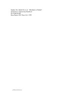
FIGURE 4.1
Position vectors in deformed and undeformed configurations.
4
e
2
e
1
X
x
undeformed
deformed
0749_Frame_C04 Page 51 Wednesday, February 19, 2003 5:33 PM
© 2003 by CRC CRC Press LLC
52
Finite Element Analysis: Thermomechanics of Solids
4.1.2 D
ISPLACEMENT
V
ECTOR
The vector
u
(
X
) represents the displacement from position
X
to
x
:
(4.1)
Now consider two close points, P and Q, in the undeformed configuration. The
vector difference
X
P
−
X
Q
is represented as a differential
d
X
with squared length
dS
2
=
d
X
T
d
X
. The corresponding quantity in the deformed configuration is
d
x
, with
dS
2
=
d
x
T
d
x
.
4.1.3 D
EFORMATION
G
RADIENT
T
ENSOR
The deformation gradient tensor
F
is introduced as
(4.2)
F
satisfies the polar-decomposition theorem:
(4.3)
in which
U
and
V
are orthogonal and ΣΣ
ΣΣ
is a positive definite diagonal tensor whose
FIGURE 4.2
Deformed and undeformed distances between adjacent points.
ds
Q'
P'
Q *
P
*
dS
u() .XxX,t =−
ddxFX F
x
X
==
∂
∂
FUV=Σ
T
,
0749_Frame_C04 Page 52 Wednesday, February 19, 2003 5:33 PM
© 2003 by CRC CRC Press LLC
Kinematics of Deformation
53
entries
λ
j
, the singular values of
F
, are called the principal stretches.
(4.4)
Based on Equation 4.3,
F
can be visualized as representing a rotation, followed
by a stretch, followed by a second rotation.
4.2 STRAIN
The deformation-induced change in squared length is given by
(4.5)
in which
E
denotes the
Lagrangian strain tensor
. Also of interest is the
Right Cauchy-
Green strain
C
=
F
T
F
=
2
E
+
I
. Note that
F
=
I
+
∂
u
/
∂
X
. If quadratic terms in
∂
u
/
∂
X
are neglected, the linear-strain tensor
E
L
is recovered as
(4.6)
Upon application of Equation 4.3,
E
is rewritten as
(4.7)
Under pure rotation
x
=
QX
,
F
=
Q
and
E
=
[
Q
T
Q
−
I
]
=
0
. The case of pure
rotation in small strain is considered in a subsequent section.
4.2.1 F
,
E
, E
L
AND u IN ORTHOGONAL COORDINATES
Let Y
1
, Y
2
, and Y
3
be orthogonal coordinates of a point in an undeformed configura-
tion, with y
1
, y
2
, y
3
orthogonal coordinates in the deformed configuration. The
corresponding orthonormal base vectors are ΓΓ
ΓΓ
1
,ΓΓ
ΓΓ
2
,ΓΓ
ΓΓ
3
and γγ
γγ
1
,γγ
γγ
2
,γγ
γγ
3
.
4.2.1.1 Deformation Gradient and Lagrangian Strain Tensors
Recalling relations introduced in Chapter 1 for orthogonal coordinates, the differential
position vectors are expressed as
(4.8)
Σ=
λ
λ
λ
1
2
3
00
00
00
ds dS d d
22
2
1
2
−= = −XFFI
TT
XEE[],
E
L
=
∂
∂
+
∂
∂
1
2
u
X
u
X
T
.
E =−
VIV
T
1
2
2
()ΣΣ
1
2
ddYH ddyhRr==
∑∑
ααα
α
ββ β
β
ΓΓγγ
0749_Frame_C04 Page 53 Wednesday, February 19, 2003 5:33 PM
© 2003 by CRC CRC Press LLC
54 Finite Element Analysis: Thermomechanics of Solids
(4.9)
in which ΓΓ
ΓΓ
β
denotes the base vector in the curvilinear system used for the undeformed
configuration.
This can be written as
(4.10)
in which Q is the orthogonal tensor representing transformation from the undeformed
to the deformed coordinate system. It follows that
from which
(4.11)
Displacement Vector
The position vectors can be written in the form R = Z
i
ΓΓ
ΓΓ
i
, r = z
j
γγ
γγ
j
. The displacement
vector referred to the undeformed base vectors is
(4.12)
Cylindrical Coordinates
In cylindrical coordinates,
(4.13)
ddyh
dy h
dy h q
q
h
H
dy
dY
HdY
q
h
H
dy
dY
HdY
r
T
T
T
=
=⋅
=
=
=∧
∑
∑∑
∑∑
∑∑∑
∑∑∑
αα α
α
αα α
ββ
αβ
αα
βα β
αβ
βα
α
ζ
α
ζ
ζζ
β
αβζ
βα
α
ζ
α
ζ
β
ζζζζ
αβζ
γ
γγ
ΓΓΓΓ
ΓΓ
ΓΓ
ΓΓΓΓ))ΓΓ
()
(,
dd q
h
H
y
Y
rQFR Q F
TTT
=
′
=
′
=
∂
∂
, [ [ ] , ]
βα βα
αζ
α
ζ
α
ζ
EFFI FFI=−=
′′
−
1
2
1
2
[][ ],
TT
[] .E
ij
ij i j
ij
h
HH
y
Y
y
Y
=
∂
∂
∂
∂
−
∑
1
2
2
βββ
β
δ
u =− =⋅[], .zZ
jji i i ji j i
qqΓΓγγΓΓ
ueee=−−+−+−[ cos( ) ] sin( ) ( ) .rRr zZ
RZ
θθ
θ
ΘΘ
0749_Frame_C04 Page 54 Wednesday, February 19, 2003 5:33 PM
© 2003 by CRC CRC Press LLC
Kinematics of Deformation 55
We now apply the chain rule to ds
2
in cylindrical coordinates:
(4.14)
in which
(4.15)
4.2.1.2 Linear-Strain Tensor in Cylindrical Coordinates
If quadratic terms in the displacements and their derivatives are neglected, then
(4.16)
ds d d dr r d dz
dr
dR
dR
R
dr
d
Rd
dr
dZ
dZ r
d
dR
dR
r
R
d
d
Rd r
d
dZ
dZ
dz
dR
dR
R
dz
d
Rd
dz
dZ
dZ
dR Rd dZ
dR
Rd
dZ
22222
2
2
2
1
1
=⋅= + +
=+ +
++ +
++ +
=
rr
C
θ
θθ θ
Θ
Θ
Θ
Θ
Θ
Θ
ΘΘ
{}
,
c
dr
dR
r
d
dR
dz
dR
ec
c
R
dr
d
r
R
d
dR
dz
d
ec
c
dr
dZ
r
d
dZ
dz
dZ
e
RR RR RR
ZZ ZZ
=
+
+
=−
=
+
+
=−
=
+
+
2
2
2
2
2
2
2
2
2
1
2
1
11 1
2
1
θ
θ
θ
()
()
ΘΘ ΘΘ ΘΘ
ΘΘΘ
==−
=
+
+
=
=
+
+
1
2
1
111
2
11
()c
c
dr
dR R
dr
d
r
d
dR
r
R
d
d
dz
dR R
dz
d
ec
c
R
dr
d
dr
dZ
r
R
d
d
r
d
dZ R
dz
d
ZZ
R RR
Z
Θ ΘΘ
Θ
ΘΘΘ
ΘΘ
θθ
θθ
ΘΘ
ΘΘ
=
=
+
+
=
dz
dZ
ec
c
dr
dZ
dr
dR
r
d
dZ
r
d
dR
dz
dZ
dz
dR
ec
ZZ
ZR ZR ZR
1
2
1
2
θθ
.
urR
u
R
uzZ
RZ
≈− ≈− ≈−
Θ
Θ
θ
,
dr
dR
du
dR
r
d
dR
R
d
dR
u
R
du
dR
u
R
dz
dR
du
dR
R
dr
dR
du
d
r
R
d
d
Ru
RR
du
d
u
RR
du
dR
dz
dR
du
d
dr
dZ
du
dZ
r
d
dZ
du
dZ
R Z
RR R Z
R
≈+ ≈
=− ≈
≈=
+
+
≈+ + ≈
≈≈
1
11
1
1111
θ
θ
θ
ΘΘΘ
ΘΘ
Θ
ΘΘ Θ Θ Θ ΘΘ
1
dzdz
dZ
du
dZ
Z
≈+1
0749_Frame_C04 Page 55 Wednesday, February 19, 2003 5:33 PM
© 2003 by CRC CRC Press LLC
56 Finite Element Analysis: Thermomechanics of Solids
giving rise to the linear-strain tensor
(4.17)
The divergence of u in cylindrical coordinates is given by ∇ ⋅ u = trace =
trace(E
L
), from which
(4.18)
which agrees with the expression given in Schey (1973).
4.2.2 VELOCITY-GRADIENT TENSOR, DEFORMATION-RATE TENSOR,
AND SPIN TENSOR
We now introduce the particle velocity v =
∂
x/
∂
t and assume that it is an explicit
function of x(t) and t. The velocity-gradient tensor L is introduced using dv = Ldx,
from which
(4.19)
Its symmetric part, called the deformation-rate tensor,
(4.20)
can be regarded as a strain rate referred to the current configuration. The correspond-
ing strain rate referred to the undeformed configuration is the Lagrangian strain rate:
(4.21)
E
L
RR
R
R
du
dR
du
dR
u
RR
u
R
du
dR
du
dZ
du
dR
u
RR
u
R
u
RR
du
d
du
dZ R
du
d
du
dR
du
dZ
du
dZ
R Z
RZ
Z
=
−+
+
−+
++
+
+
∂
∂
∂
∂
1
2
11
2
1
2
111
2
1
1
2
1
2
ΘΘ
ΘΘ Θ Θ
Θ
ΘΘ
11
R
du
d
du
dZ
ZZ
Θ
.
d
d
u
r
∇⋅ = + + +u
du
dR
u
RR
du
d
du
dZ
RR Z
1
Θ
Θ
,
L
v
x
v
X
X
x
FF
1
=
=
=
−
d
d
d
d
d
d
˙
.
DLL
T
=+
1
2
[],
˙
[
˙˙
]
[
˙˙
]
.
E =+
=+
=
−−
1
2
1
2
FF FF
FFFFFF
FDF
TT
T1TT
T
0749_Frame_C04 Page 56 Wednesday, February 19, 2003 5:33 PM
© 2003 by CRC CRC Press LLC
Kinematics of Deformation 57
The antisymmetric portion of L is called the spin tensor W:
(4.22)
Suppose the deformation consists only of a time-dependent, rigid-body motion:
(4.23)
Clearly, F = Q and E = 0. Furthermore,
(4.24)
which is antisymmetric since .
Hence, D = 0 and , thus explaining the name of W.
4.2.2.1 v, L, D, and W in Orthogonal Coordinates
The velocity v(y, t) in orthogonal coordinates is given by
(4.25)
Based on what we learned in Chapter 1, with v denoting the velocity vector in
orthogonal coordinates,
(4.26)
Of course,
4.2.2.2 Cylindrical Coordinates
The velocity vector in cylindrical coordinates is
(4.27)
WLL
T
=−
1
2
[].
xQXb QQI
T
() () (), () () .tt t tt=+ =
LQQ
T
=
˙
,
0 I QQ QQ QQ QQ QQ
TTTTTT
== =+=+
˙
[]
˙˙˙
(
˙
)
•
WQQ
T
=
˙
vy
r
( , ) , .t
d
dt
vvh
dy
dt
== =
∑
αα
α
αα
α
γγ
[] .L
βα
βα
αα
ββα
δ
=
=
∂
∂
+
d
dh
v
y
v
j
j
j
j
v
r
1
c
c
αβ
α
αβ β
β
α
β
δ
αβ
αβ
j
k
j
k
h
h
h
x
yy
y
x
j
j
=−
=
∂
∂∂
∂
∂
1
1
2
()
[ ] [[ ] [ ] ] [ ] [[ ] [ ] ].,DLLWLL
βα βα αβ βα βα αβ
=+ =−
1
2
1
2
ve e e
eee
=+ +
=++
dr
dt
r
d
dt
dz
dt
vv v
rz
rr zz
θ
θ
θθ
.
0749_Frame_C04 Page 57 Wednesday, February 19, 2003 5:33 PM
© 2003 by CRC CRC Press LLC
58 Finite Element Analysis: Thermomechanics of Solids
Observe that
(4.28)
Converting to matrix-vector notation, we get
(4.29)
4.2.2.3 Spherical Coordinates
Now
(4.30)
Next,
(4.31)
ddv dv dv vd vd
dv v d dv v d dv
rr zz r r
rr r zz
ve e e e e
eee
=++++
=− ++ +
θθ θ θ
θθθ
θθ
[][].
d
dv
dr r
dv
d
dv
dz
v
r
dv
dr r
dv
d
dv
dz
v
r
dv
dr r
dv
d
dv
dz
dv
dr r
dv
rrr
zz
rr
dr rd dz rd
dr rd dz rd
dr rd dz
dr
rd
dz
r
z
v
LL
=+
==
++−
++
++
1
1
1
1
θ
θ
θ
θθ
θθ
θ
θ
θ
θθθ
,
dd
v
r
dv
dz
dv
dr r
dv
d
v
r
dv
dz
dv
dr r
dv
d
dv
dz
r
zzz
r
θ
θ
θ
θ
θθ θ
−
+
1
1
.
ve e e
eee
eeee
eee
eeee
=+ +
=++
=++
=− +
=− + +
dr
dt
r
d
dt
r
d
dt
vv v
r
rr
r
cos
cos (cos sin ) sin
sin cos
sin (cos sin ) cos .
φ
θφ
φθ θ φ
θθ
φθ θ φ
θ
φ
θθ
φφ
θ
φ
12 3
12
12 3
′
==
′
=−
−−
vQv v v eee
Q
,, ,,
cos cos cos sin sin
sin cos
sin cos sin sin cos
referred to
v
v
v
r
θ
φ
φθ φθ φ
θθ
φθ φθ φ
123
0
0749_Frame_C04 Page 58 Wednesday, February 19, 2003 5:33 PM
© 2003 by CRC CRC Press LLC
Kinematics of Deformation 59
(4.32)
Recall that
(4.33)
Thus, it follows that
(4.34)
and
(4.35)
Finally,
(4.36)
ddd
dd d
dv
dv
dv
r
r
vQQv* QQv
v* QQ v v* e e e
TT
T
=+
=+ =
referred to ,,,
θ
φ
θ
φ
d
dt
d
dt
d
dt
Q
Q
()
()
cos
cos sin
sin
.
θ
θ
φ
φφ
φ
θφ
T
=−
−
+
−
00
0
00
001
000
100
d
r
rd
r
rdQQ
T
=−
−
+
−
1
00
0
00
1
001
000
100
cos
cos
cos sin
sin
cos
φ
φ
φφ
φ
φθ φ
d
vd vd
vd vd
vd vd
r
vv
vv
vv
dr
rd
rd
r
r
r
r
QQ v
T
=
+
−+
−−
=−+
−−
cos
cos sin
sin
tan
tan
cos .
φθ φ
φθ φθ
φθ φ
φ
φ
φθ
φ
θ
φ
φ
θ
θ
φ
φ
θ
1
0
00
0
dv
dv
dv
dv
dr
rd
rd
r
dv
dr r
dv
dr
dv
d
dv
dr r
dv
dr
dv
d
dv
dr r
dv
dr
dv
d
rrr
* =
=
θ
φ
φθ φ
φθ φ
φθ φ
θθθ
φφφ
φθ
φ
11
11
11
cos
cos
cos
cos
0749_Frame_C04 Page 59 Wednesday, February 19, 2003 5:33 PM
© 2003 by CRC CRC Press LLC
60 Finite Element Analysis: Thermomechanics of Solids
and
(4.37)
The divergence of v is given by trace(L), thus,
(4.38)
which is again in agreement with Schey (1973).
4.3 DIFFERENTIAL VOLUME ELEMENT
The volume spanned by the differential-position vector dR is given by the vector
triple-product
(4.39)
The vectors dX
i
deform into dx
j
= e
j
dX
i
. The deformed volume is now readily
verified to be
(4.40)
and J is called the Jacobian. To obtain J for small strain, we invoke invariance and
to find
(4.41)
L =
+−+
−−
=
dv
dr r
dv
dr
dv
d
dv
dr r
dv
dr
dv
d
dv
dr r
dv
dr
dv
d
dv
dr
rrr
r
r
vv
vv
vv
r
r
11
11
11
1
0
00
0
cos
cos
cos
tan
tan
φθ φ
φθ φ
φθ φ
θθθ
φφφ
θ
φ
φ
θ
φ
φ
111
11
11
r
dv
d
v
rr
dv
d
v
r
dv
dr r
dv
d
vv
rr
dv
d
dv
dr r
dv
d
v
rr
dv
d
v
r
rr
r
r
cos
cos
tan
cos
tan
.
φθ φ
φθ
φ
φ
φθ
φ
φ
θ
φ
θθ
φ
θ
φφ
θ
φ
++
−
−−
−
∇⋅ = + −
−
+v
dv
dr r
dv
d
vv
rr
dv
d
r
r
11
cos
tan
,
φθ
φ
φ
θ
φφ
dV d d d d d d
d dX d dX d dX
0123123
111 2 22 3 33
=⋅×=
== =
XX X XXX
XeX eX e .
dx
d
j
i
x
dV d d d
JdV J
=⋅×
===
xx x
FC
12 3
0
1
2
,()(), det det
J = det()C
det det
1
2
1
2
2
12 12 12
() [ ]
()( )( ),
CI=+
=+ + +
E
EE E
I II III
0749_Frame_C04 Page 60 Wednesday, February 19, 2003 5:33 PM
© 2003 by CRC CRC Press LLC
Kinematics of Deformation 61
in which E
I
, E
II
, E
III
are the eigenvalues of E
L
, assumed to be much less that unity.
The linear-volume strain follows as
(4.42)
using the approximation 1 + x/2 if x << 1.
The time derivative of J is prominent in incremental formulations in continuum
mechanics. Recalling that ,
(4.43)
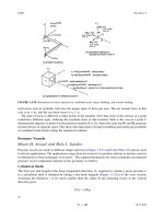
4.4 DIFFERENTIAL SURFACE ELEMENT
Let dS denote a surface element in the deformed configuration, with exterior unit
normal n, as illustrated in Figure 4.3. The corresponding quantities from the refer-
ence configuration are dS
0
and n
0
. A surface element dS obeys the transformation
(Chandrashekharaiah and Debnath, 1994):
(4.44)
from which we conclude that
(4.45)
e det
EE E
tr
vol
I II III
L
=−
=+ + + + −
≈
1
2
1
12 1
()
()
(),
C
quadratic terms
E
1+≈x
JI=
3
d
dt
J
J
dI
dt
J
tr
J
tr
J
tr
J
tr tr
Jtr
Jtr
=
=
=+
=+
=+
=
+
=
−
−−
−−−
−−−
−−
1
2
2
2
2
2
2
3
(
˙
)
([
˙˙
])
(
˙˙
)
[(
˙
)(
˙
)]
˙˙
CC
F F FF FF
FF FF FF
FF FF FF
FF F F
1
1TT T
11TT
11TT
1TT
(().D
nFn
T
dS J dS=
−
00
,
dS J dS==
−
−
−
nC n n
Fn
nC n
T1
T
T1
000
0
00
.
0749_Frame_C04 Page 61 Wednesday, February 19, 2003 5:33 PM
© 2003 by CRC CRC Press LLC
62 Finite Element Analysis: Thermomechanics of Solids
During deformation, the surface normal changes direction, a fact which is impor-
tant, for example, in contact problems. In incremental variational methods, we
consider the differential and d(ndS):
(4.46)
However, recalling Equation 4.43,
(4.47)
Also, since d(F
T
F
−T
) = 0, then
(4.48)
Finally, we have
(4.49)
Next, we find with some effort that
(4.50)
FIGURE 4.3 Surface patches in undeformed and deformed configurations.
dX
1
dx
1
dS
0
n
0
n
dx
2
dS
dX
2
d
dt
n
d
dt
dS
dJ
dt
dS J
d
dt
dS[] .nFn
F
n
T
T
=+
−
−
00 00
dJ
dt
Jtr
dJ
dt
dS tr J dS
tr dS
=
=
=
−−
()
()
() .
D
Fn DFn
Dn
TT
00 00
d
dt
d
dt
T
T
T
T
TT
F
F
F
F
LF
−
−−
−
=−
=− .
d
dt
[]
[() ] .
n
DI L n
dS
tr dS
T
=−
d
dt
d
dt
d
dt
nF
n
nC n
Fn
nC n
nn
nC n
nDnI L n
T
T
T
T
T
T1
TT
C
=−
=−
−
−
−
−
−
−
0
00
0
00
00
00
11
1
[( ) ] .
0749_Frame_C04 Page 62 Wednesday, February 19, 2003 5:33 PM
© 2003 by CRC CRC Press LLC
Kinematics of Deformation 63
4.5 ROTATION TENSOR
Elementary manipulation furnishes
(4.51)
in which the antisymmetric rotation tensor ωω
ωω
appears:
. (4.52)
Consider pure rotation with small angle
θ
:
(4.53)
thus,
(4.54)
(4.55)
Evidently, the normal strains do not vanish, but are second-order in
θ
, while ωω
ωω
is first-order in
θ
. Under the assumption of small deformation, nonlinear terms are
neglected so that E
L
is regarded as vanishing.
d
d
d
d
d
L
u
u
X
X
X
=
=+[],E ωω
ωω=
∂
∂
−
∂
∂
1
2
u
X
u
X
T
xX
X
=−
≈
−
−−
cos sin
sin cos
,
θθ
θθ
θ
θ
θ
θ
0
0
001
10
10
001
2
2
2
2
uXX=
−
−
+−
θ
θ
θ
θ
2
2
2
2
00
00
000
0
00
000
0
E
L
=
−
−
=−
θ
θ
θ
θ
2
2
2
2
00
00
000
0
00
000
,.
0
ωω
0749_Frame_C04 Page 63 Wednesday, February 19, 2003 5:33 PM
© 2003 by CRC CRC Press LLC
64 Finite Element Analysis: Thermomechanics of Solids
Consider as a second example the following derivation in which the sides of the
unit square rotate toward each other by 2
θ
.
The deformation can be described by the relations
(4.56)
from which we conclude that
(4.57)
Upon neglecting quadratic terms, we conclude that linear-shear strain is a mea-
sure of how much the axes rotate toward each other, while the rotation tensor is a
measure of how much the axes rotate in the same sense.
4.6 COMPATIBILITY CONDITIONS FOR E
L
AND D
The following paragraphs present the compatibility equations for the linear-strain
tensor, allowing E
L
to be integrated to produce a displacement field u(X), which is
unique to within a rigid-body motion. It should be evident that a parallel argument
produces exactly the same result for the velocity vector v(x) starting from a given
deformation-rate tensor D(x).
FIGURE 4.4 Element in undeformed and deformed configurations.
Y
L
L
L
L
X
θ
θ
xXYXY
yX YX Y
=− + ≈−
+
=+− ≈+−
( cos ) sin
sin ( cos ) ,
11
2
11
2
2
2
θθ
θ
θ
θθθ
θ
E
L
=
−
−
θ
θ
θ
θ
2
2
2
2
0
0
000
.
0749_Frame_C04 Page 64 Wednesday, February 19, 2003 5:33 PM
© 2003 by CRC CRC Press LLC
Kinematics of Deformation 65
There are two major “paths” to solutions of problems in continuum mechanics.
For example,
Assume/approximate u. Apply the strain-displacement relations to estimate E,
apply the stress-strain relations to estimate S, and then apply equilibrium
relations to obtain the field equation. Solve the field equation applying
boundary conditions and constraints.
Assume/approximate S, and then estimate E using the strain-displacement
relations. Apply compatibility relations to obtain the field equation, and
then solve the field equation and boundary conditions and constraints.
To understand the second solution path, we focus on the following compatibility
relation. Suppose the linear strains are known as functions of the position X. Under
what circumstances can the strain-displacement relations be integrated to produce
a displacement field that is unique to within a rigid-body displacement? Recall that
(4.58)
Evidently, E
L
is only part of the derivative of u. In 2-D rectilinear coordinates,
we will see that the compatibility equation, guaranteeing unique u to within a rigid-
body motion, is given by:
(4.59)
The proof of the compatibility equation is as follows. We consider a path in the
physical (X
1
, X
2
, X
3
) space, along which the arc length is denoted by
λ
. Accordingly,
the position vector X is a function of
λ
. The integral of du, taken from
λ
= 0 to
λ
* is
(4.60)
The term u(0) can be interpreted as the rigid-body translation. The first integral
can be evaluated since E(X) and X(
λ
) are given functions. The second integral can
be rewritten using an elementary transformation as
(4.61)
d
d
d
d
d
L
u
u
X
X
X
=
=+[]E ωω
∂
∂∂
=
∂
∂
+
∂
∂
2
12
12
2
11
2
2
2
22
1
2
1
2
E
xx
E
x
E
x
uX u
u
X
X
uXXXX
X
XX
( ( *)) ( )
( ) ( ( *)) ( ) .
(*)
(*)(*)
λ
λ
λ
λλλ
=+
=+ +
∫
∫∫
0
0
0
00
d
d
d
ddE ωω
ωωωω() ( * )( * ).
(*)
(*)
XX XXXX
X
X
dd
0
0
λ
λ
∫∫
=− − −
0749_Frame_C04 Page 65 Wednesday, February 19, 2003 5:33 PM
© 2003 by CRC CRC Press LLC
66 Finite Element Analysis: Thermomechanics of Solids
Note the following:
(4.62)
Consequently, integration by parts furnishes
(4.63)
The term ωω
ωω
(X(0))(X(
λ
*) − X(0)) can be identified as a rigid-body rotation since
the rotation tensor ωω
ωω
(X(0)) is independent of position. We now focus on the second
term. Now that rigid-body translation and rotation have been accommodated, the
integral should give a unique value regardless of the path. Consider two paths, path
1 and path 2, from
λ
= 0 to
λ
*. The integral over these paths should produce the same
unique values. Therefore, the closed path 0 to
λ
* along path 1 followed by
λ
* to 0 in
a negative sense along path 2 should vanish. Furthermore, path 1 and path 2 are
arbitrary, except for terminating at the same points. It follows that along any closed path
(4.64)
Let us now write ωω
ωω
(X) as ωω
ωω
(X) = {ωω
ωω
1
(X) ωω
ωω
2
(X) ωω
ωω
3
(X)}, in which ωω
ωω
i
denotes
the vector corresponding to the i
th
column of ωω
ωω
. The compatibility condition can
now be written as
(4.65)
For a suitable differential function Ψ(X), the condition for ͛ΨΨ
ΨΨ
⋅ dX = 0 over
an arbitrary contour is that the curl of Ψ vanishes, from which we express the
compatibility conditions as
(4.66)
ddd
dd
d
d
d
d
TT T
TT
T
[()(*)]()(*)[(*) (*)]
()( * )[(* ) (* )]
()( * ) ( * )
(* )
(* )
(* )
ωωωωωω
ωωωω
ωω
ωω
XXX XXX XX XX
XX X X X X X
XX X X X
XX
XX
XX
−= −+ − −
=−−−−
=−−−
−
−
−
T
.
−−=−
+−
−
−
−
∫
∫
−
ωωωω
ωω
( ) ( ) ( ( ))( ( *) ( ))
(* )
(* )
(* )
(* ).
(*)
() ()
*
XX*X X X X
XX
XX
XX
XX
X
XX
d
d
d
d
T
T
λ
λ
λ
0
0
0
00
(* )
(* )
(* )
(* ) .XX
XX
XX
XX0−
−
−
−=
∫
TT
d
d
d
ωω
(* )
(* )
(* )
(* ) , ,,.XX
XX
XX
XX−
−
−
−= =
∫
T
j
d
d
dj
ωω
0123
∇× −
−
==(* )
()
(* )
,,,.XX
X
XX
T
d
d
j
j
ωω
0123
0749_Frame_C04 Page 66 Wednesday, February 19, 2003 5:33 PM
© 2003 by CRC CRC Press LLC
Kinematics of Deformation 67
This can be expanded at considerable effort to derive 81 compatibility equations,
including Equation 4.59.
4.7 SAMPLE PROBLEMS
1. Referring to Figure 4.5, determine u, F, J, and E as functions of X and Y.
Use H = 1.0, W = 1.0, a = 0.1, b = 0.1, c = 0.3, d = 0.2, e = 0.2, f = 0.1.
Assume a unit thickness in the Z-direction in both the deformed and
undeformed configurations.
Solution: Since straight sides are deformed into straight sides, the deformation
pattern can be assumed in the form
and it is necessary to determine
α
,
β
,
γ
,
δ
,
ε
, and
ζ
from the coordinates
of the vertices in the deformed configuration.
After elementary manipulation,
FIGURE 4.5 Plate elements in undeformed and deformed states.
xXYXYyXYXY=++ =++
αβγ δεζ
,
At
At
At
(,) ( ,) :
(,) (, ) :
(,) ( , ):
XY W W a W b W
XY H e H H f H
X Y W H W c H H WH H d W H WH
=+= =
== +=
=+=+++=++
0
0
αδ
βε
αβγ δεζ
αβ δ
εγ ζ
=+ = = = = =
=+ = =
+− + −
==
+−− +
=
111 02 01
112 04 0
a
W
e
H
b
W
f
H
Wc Wa e
WH
Hdb H f
WH
.
.
()
.
()
.
YY
W
W
H
X
X
undeformed plate deformed plate
H
a
b
d
c
e
f
0749_Frame_C04 Page 67 Wednesday, February 19, 2003 5:33 PM
© 2003 by CRC CRC Press LLC
68 Finite Element Analysis: Thermomechanics of Solids
The 2 × 2 deformation gradient tensor F and its determinant are now:
.
The displacement vector is
The Lagrangian strain E = [F
T
F − I] is
2. Figure 4.6 shows a square element at time t and at t + dt. Estimate L, D,
and W at time t. Use a = 0.1dt, b = 1 + 0.2dt, c = 0.2dt, d = 1 + 0.4dt,
e = 0.05dt, f = 0.1dt, g = 1 − 0.1dt, h = 1 + 0.5dt. Assume a unit thickness
in the Z-direction in both the deformed and undeformed configurations.
FIGURE 4.6 Element experiencing rigid body motion and deformation.
F =
++
++
=
++
=+ −
αγ βγ
δζ εζ
YX
YX
YX
JYX
11 04 02 04
01 12
13 048 004
.
u =
−
−
=
−
()
++
+−
()
+
=
++
+
xX
yY
XYXY
XYXY
XYXY
XY
αβγ
δε ζ
1
1
01 02 04
01 02
.
1
2
E =
+
+
++
−
=
++ +++
+
1
2
11 04 01
02 04 12
11 04 02 04
01 12
1
2
10
01
011 044 008 017 022 004 008
017 0
2
.
.
. . .
.
Y
X
YX
YY XYXY
. . . . .22 0 04 0 08 0 24 0 08 0 08
2
XYXY XX++ ++
YY
X
X
1
1
a
e
g
c
d
h
f
b
element at time t element at time t+dt
0749_Frame_C04 Page 68 Wednesday, February 19, 2003 5:33 PM
© 2003 by CRC CRC Press LLC
Kinematics of Deformation 69
Solution: First, represent the deformed position vectors in terms of the unde-
formed position vectors using eight coefficients determined using the given
geometry. In particular,
Following procedures analogous to Problem 1, we find:
The velocities can be estimated using v
x
≈ and v
y
≈ , from which
The tensors L, D, and W are now readily found as:
4.8 EXERCISES
1. Consider a one-dimensional deformation in which x = (1 +
λ
)X. What
value of
λ
is the linear-strain
ε
L
error by 5% relative to the Lagrangian
strain E? Use the error measure
2. A 1 × 1 square plate has a constant (2 × 2) Lagrangian-strain tensor E.
What is the deformed length of the diagonal? What is the volume change?
xXYXYyXYXY=+ + + =+ + +
αβ γ δ εζ η θ
.
αε
βζ
γη
δθ
==
=+ =
==−
=− =−
01 005
102 01
02 1 01
05 005
dt dt
dt dt
dt dt
dt dt
xX
dt
−
yY
dt
−
vXYXY
vXYXY
x
y
=+ + −
=+ −−
01 02 02 05
005 01 01 005
. .
L
D
W
=
−−
−−−
=
−−−
−− −−
=
−− +
02 05 02 05
01 005 01 005
02 05 015 025 0025
015 025 0025 01 005
0 0 4 0 25 0 025
04
. . .
.
.
.
YX
YX
YXY
XY X
XY
++−
0 25 0 025 0
.
XY
error
L
=
−EE
E
.
0749_Frame_C04 Page 69 Wednesday, February 19, 2003 5:33 PM
© 2003 by CRC CRC Press LLC
70 Finite Element Analysis: Thermomechanics of Solids
If the linear strain E
L
is now approximated as E, what is the diagonal and
what is the volume change? Take
3. Verify that the expressions in the text for F and E in cylindrical coordinates
are consistent with the equation
in which Q is the orthogonal tensor representing transformation from the
undeformed to the deformed coordinate system, and also with
4. Obtain expressions for u, F, E, and E
L
in spherical coordinates.
5. For cylindrical coordinates, determine the Lagrangian strain in the fol-
lowing two cases:
6. In spherical coordinates, determine the Lagrangian strain for pure radial
expansion.
7. Obtain v, L, D, and W in spherical coordinates.
8. For cylindrical coordinates, find L, D, and W for the following flows:
9. In spherical coordinates, find L, D, and W for pure radial expansion:
E =
01 005
005 01
.
FQF Q F
TT
=
′
=
′
=
∂
∂
,[ [ , ] ]
βα βα
αζ
α
ζ
α
ζ
q
h
H
y
Y
[] .E
ij
ij i j
ij
h
HH
y
Y
y
Y
=
∂
∂
∂
∂
−
∑
1
2
2
βββ
β
δ
( ) Pure radial expansion:
( ) Torsion:
arRzZ
brRZzZ
===
==+ =
λθ
θλ
,,
,,
Θ
Θ
rR===
λθ φ
,, ΘΦ
(a) pure radial flow:
(b) pipe flow:
(c) cylindrical flow:
(d) torsional flow:
vfr v v
vvvfr
vvfrv
vvfzv
rz
rz
rz
rz
===
===
===
===
(), ,
,,()
,(),
,(),
θ
θ
θ
θ
00
00
00
00
vfr v v
r
===(), ,
θ
φ
00
0749_Frame_C04 Page 70 Wednesday, February 19, 2003 5:33 PM
© 2003 by CRC CRC Press LLC
Kinematics of Deformation 71
10. For linear strain in rectilinear coordinates and 2-D, the compatibility
relation is
Find the implications of this relation for a linear-strain field assumed to
be given by
11. Consider a square L × L plate (undeformed configuration) with linear
strains
Assuming that the origin does not move, find the deformed position of
(X,Y) = (L,L).
∂
∂∂
=
∂
∂
+
∂
∂
2
12
12
2
11
2
2
2
22
1
2
1
2
E
xx
E
x
E
x
.
EaXaXYaY
EbXbXYbY
EcXcXYcY
11 1
2
23
2
22 1
2
23
2
12 1
2
23
2
=++
=++
=++.
EaaXaY
EbbXbY
EccXcY
11 1 2 3
22 1 2 3
12 1 2 3
=+ +
=+ +
=+ + .
0749_Frame_C04 Page 71 Wednesday, February 19, 2003 5:33 PM
© 2003 by CRC CRC Press LLC