Finite Element Analysis - Thermomechanics of Solids Part 6 ppt
Bạn đang xem bản rút gọn của tài liệu. Xem và tải ngay bản đầy đủ của tài liệu tại đây (414.57 KB, 12 trang )
95
Stress-Strain Relation and
the Tangent-Modulus
Tensor
6.1 STRESS-STRAIN BEHAVIOR: CLASSICAL
LINEAR ELASTICITY
Under the assumption of linear strain, the distinction between the Cauchy and Piola-
Kirchhoff stresses vanishes. The stress is assumed to be given as a linear function
of linear strain by the relation
(6.1)
in which
c
ijkl
are constants and are the entries of a 3
×
3
×
3
×
3 fourth-order tensor,
C
. If
T
and
E
L
were not symmetrical,
C
might have as many as 81 distinct entries.
However, due to the symmetry of
T
and
E
L
there are no more than 36 distinct entries.
Thermodynamic arguments in subsequent sections will provide a rationale for the
Maxwell
relations:
(6.2)
It follows that
c
ijkl
=
c
klij
, which implies that there are, at most, 21 distinct coeffi-
cients. There are no further arguments from general principles for fewer coefficients.
Instead, the number of distinct coefficients is specific to a material, and reflects the
degree of symmetry in the material. The smallest number of distinct coefficients is
achieved in the case of isotropy, which can be explained physically as follows.
Suppose a thin plate of elastic material is tested such that thin strips are removed
at several angles and then subjected to uniaxial tension. If the measured stress-strain
curves are the same and independent of the orientation at which they are cut, the
material is isotropic. Otherwise, it exhibits anisotropy, but may still exhibit limited
types of symmetry, such as transverse isotropy or orthotropy. The notion of isotropy
is illustrated in Figure 6.1.
In isotropic, linear-elastic materials (which implies linear strain), the number of
distinct coefficients can be reduced to two,
m
and
l
, as illustrated by Lame’s equation,
(6.3)
6
TcE
ij
ijkl kl
L
=
()
,
∂
∂
=
∂
∂
T
E
T
E
ij
kl
kl
ij
.
TEE
ij ij
L
kk
L
ij
=+2
µλδ
() ()
.
0749_Frame_C06 Page 95 Wednesday, February 19, 2003 5:06 PM
© 2003 by CRC CRC Press LLC
96
Finite Element Analysis: Thermomechanics of Solids
This can be inverted to furnish
(6.4)
The classical elastic modulus E
0
and Poisson’s ratio
n
represent response
under
uniaxial tension only
, provided that
T
11
=
T
,
T
ij
= 0. Otherwise,
(6.5)
It is readily verified that
(6.6)
from which it is immediate that
(6.7)
Leaving the case of uniaxial tension for the normal (diagonal) stresses and
strains, we can write
(6.8)
(6.9)
FIGURE 6.1
Illustration of isotropy.
1
2
3
4
T
21
3
4
E
ET T
ij
L
ij
kk
ij
()
.=−
+
1
223
µ
λ
µλ
δ
E ==−=−
T
E
E
E
E
E
L
L
L
L
L
11
11
22
11
33
11
()
()
()
()
()
.
ν
11
2
1
23
1
22 3E
E
=−
+
=
+
µ
λ
µλ
ν
µ
λ
µλ
,
1
2
1
µ
ν
=
+
E
,
ETTT
TTT
L
11 11 22 33
11 22 33
1
2
1
23
1
22 3
1
()
()
[ ( )],
=−
+
−
+
+
=−+
µ
λ
µλ µ
λ
µλ
ν
E
ETTT
L
22 22 33 11
1
()
[ ( )],=−+
E
ν
0749_Frame_C06 Page 96 Wednesday, February 19, 2003 5:06 PM
© 2003 by CRC CRC Press LLC
Stress-Strain Relation and the Tangent-Modulus Tensor
97
and
(6.10)
and the off-diagonal terms satisfy
(6.11)
6.2 ISOTHERMAL TANGENT-MODULUS TENSOR
6.2.1 C
LASSICAL
E
LASTICITY
Under small deformation, the fourth-order tangent-modulus tensor
D
in linear elas-
ticity is defined by
(6.12)
In linear isotropic elasticity, the stress-strain relations are written in the Lame’s
form as
(6.13)
Using Kronecker Product notation from Chapter 2, this can be rewritten as
(6.14)
from which we conclude that
(6.15)
6.2.2 C
OMPRESSIBLE
H
YPERELASTIC
M
ATERIALS
In isotropic hyperelasticity, which is descriptive of compressible rubber elasticity,
the 2
nd
Piola-Kirchhoff stress is taken to be derivable from a strain-energy function
that depends on the principal invariants
I
1
,
I
2
,
I
3
of the Right Cauchy-Green strain
tensor:
(6.16)
ETTT
L
33 33 11 22
1
()
[ ( )],=−+
E
ν
ETETET
LLL
12 12 23 23 31 31
111
() () ()
.=
+
=
+
=
+
ννν
E
E
E
ddTDE=
L
.
TE E=+2
µλ
LL
Itr().
VEC VEC()TE=⊗+[](),2
µλ
II ii
T
L
D =⊗+ITEN22 2().
µλ
II ii
T
S
EC
s
e
sSeEcC
== ==
===
d
d
d
d
d
d
d
d
(a)
(b)
ww ww
VEC VEC VEC
22
T
c
((())).
0749_Frame_C06 Page 97 Wednesday, February 19, 2003 5:06 PM
© 2003 by CRC CRC Press LLC
98
Finite Element Analysis: Thermomechanics of Solids
Now,
(6.17)
From Chapter 2,
(6.18)
The tangent-modulus tensor
D
o
, referred to the undeformed configuration, is
given by
(6.19)
and now
(6.20)
Finally,
(6.21)
In deriving
A
3
we have taken advantage of the Cayley-Hamilton theorem (see
Chapter 2).
sn n
T
==
∂
∂
=
∂
∂
2
φφ
ii i
i
c
,, .
w
i
i
I
I
nnin
1
121 3 3
==−=
−
ic CI VEC I().
dSDE s D E==
oo
TENdd )d22( ,
TEN
o
22( )
d
d
D
c
=+ =44
φφ
ij i j i i i
i
nn A A
n
T
,.
A
A
A
1
22
1
9
3
1
3
21
2
2
1
==
=
=−
=−
=
=−+
=−+⊕
=−−++⊕
−
d
d
(a)
d
d
d
d
[
(b)
d
d
d
d
(c)
i
0
i
ii I
c
i
in i
ii I i i
T
T
TT
T
9
TT
c
c
c
c
C
c
cC
cCC
cc CC
I
I
VEC I
I I VEC
I
]
[()]
[()]
[][ ]
0749_Frame_C06 Page 98 Wednesday, February 19, 2003 5:06 PM
© 2003 by CRC CRC Press LLC
Stress-Strain Relation and the Tangent-Modulus Tensor
99
6.3 INCOMPRESSIBLE AND NEAR-INCOMPRESSIBLE
HYPERELASTIC MATERIALS
Polymeric materials, such as natural rubber, are often nearly incompressible. For
some applications, they can be idealized as incompressible. However, for applica-
tions involving confinement, such as in the corners of seal wells, it may be necessary
to accommodate the small degree of incompressibility to achieve high accuracy.
Incompressibility and near-incompressibility represent
internal constraints
. The
principal (e.g., Lagrangian) strains are not independent, and the stresses are not
determined completely by the strains. Instead, differences in the principal stresses
are determined by differences in principal strains (Oden, 1972). An additional field
must be introduced to enforce the internal constraint, and we will see that this internal
field can be taken as the hydrostatic pressure (referred to the current configuration).
6.3.1 I
NCOMPRESSIBILITY
The constraint of incompressibility is expressed by the relation
J
=
1. Now,
(6.22)
and consequently,
(6.23)
The constraint of incompressibility can be enforced using a Lagrange multiplier
(see Oden, 1972), denoted here as
p
. The multiplier depends on
X
and is, in fact,
the additional field just mentioned. Oden (1972) proposed introducing an augmented
strain-energy function,
w
′
, similar to
(6.24)
in which
w
is interpreted as the conventional strain-energy function, but with depen-
dence on
I
3
(
=
1) removed. are called the deviatoric invariants. For reasons
to be explained in a later chapter presenting variational principles, this form serves
J
I
=
=
=
=
=
det
det ( )
det( )det( )
det ( )
,
F
F
FF
FF
2
2
3
T
T
I
3
1= .
′
=
′′
−−
′
=
′
=wwII pI I
I
I
I
I
I
() () ,
//
12 3 1
1
2
2
1
2
1
3
13
3
23
,,,
′′
II
12
and
0749_Frame_C06 Page 99 Wednesday, February 19, 2003 5:06 PM
© 2003 by CRC CRC Press LLC
100
Finite Element Analysis: Thermomechanics of Solids
to enforce incompressibility, with
S
now given by
(6.25)
To convert to deformed coordinates, recall that
S
= J
F
−
1
T
F
−
T
. It is left to the
reader in an exercise to derive in which
(6.26)
in which It follows that
p
=
−
tr
(
T
)
/
3 since
(6.27)
Evidently, the Lagrange multiplier enforcing incompressibility is the “true”
hydrostatic pressure.
Finally, the tangent-modulus tensor is somewhat more complicated because d
S
depends on d
E
and d
p
. We will see in subsequent chapters that it should be defined
as
D
∗
using
(6.28)
Example: Uniaxial Tension
Consider the Neo-Hookean elastomer satisfying
(6.29)
s
e
cc
=
∂
′
∂
=
′′
+
′′
−
′
=
∂
∂
′
′
=
∂
∂
′
′
=
∂
′
∂
′
=
∂
′
∂
w
p
w
I
w
I
II
22
12233
1
1
2
2
1
1
2
2
φφ
φφ
1
nnn
nn
TT
I
.
′′
ψψ
12
and
tmm==
′′
+
′′
−VEC p()T 22
11 2 2
ψψ
i
im im
TT
′
=
′
=
12
00 and .
tr
p
p
p
()
.
T =
=
′′
+
′′
−
=−
=−
it
im im ii
ii
T
T
1
TT
T
22
3
122
ψψ
TEN
p
p
22( )D
s
e
s
s
∗
=
−
d
d
d
d
d
d
T
0
d
d
d
d
s
e
s
=
′′
+
′′
+
′′ ′
+
′′′
+
′′ ′
+
′′ ′
=−
4
1 1 2 2 11 1 1 12 1 2
21 2 1 22 2 2
33
[()()
() ()]
.
φφ φ φ
φφ
A A nn nn
nn nn
TT
TT
p
In
wI=−
[]
=
α
I and subject to
13
31.
0749_Frame_C06 Page 100 Wednesday, February 19, 2003 5:06 PM
© 2003 by CRC CRC Press LLC
Stress-Strain Relation and the Tangent-Modulus Tensor
101
We seek the relation between
s
1
and
e
1
, which will be obtained twice: once by
enforcing the incompressibility constraint
a priori
, and the second by enforcing the
constraint
a posteriori
.
a priori
: Assume for the sake of brevity that
e
2
=
e
3
.
I
3
=
1 implies that
. The strain-energy function now is The stress,
s
1
, is
now found as
(6.30)
a posteriori
: Use the augmented function
(6.31)
Now
(6.32)
Thus, it follows that We conclude that
(6.33)
cc
21
1= / wc
c
=+−
α
[].
1
1
2
3
s
w
cc
1
11
32
221
1
==−
d
d
α
/
.
′
=−− −wI
p
I
α
[][].
13
3
2
1
s
w
c
pc
s
w
c
pc
s
w
c
pc
w
p
I
1
1
1
2
2
2
3
3
3
3
22
022
022
001
=
′
=−
==
′
=−
==
′
=−
=
′
=→ =
d
d
d
d
d
d
d
d
α
α
α
/
/
/
.
cc c pc
23 1 2
12== =/ and /
α
.
spc
c
c
pc
c
c
c
11
2
1
2
2
1
1
32
2
2
21
21
1
=−
=−
=−
=−
α
α
α
α
/
/
.
/
0749_Frame_C06 Page 101 Wednesday, February 19, 2003 5:06 PM
© 2003 by CRC CRC Press LLC
102
Finite Element Analysis: Thermomechanics of Solids
a posteriori with deviatoric invariants
: Consider the augmented function with
deviatoric invariants:
(6.34)
Hence,
c
2
=
c
3
. Furthermore,
(6.34e)
Equation 6.34 now implies that
(6.35)
and substitution into Equation 6.34b furnishes
(6.36)
as in the
a priori
case and in the first
a posteriori
case. Now, the Lagrange multiplier
p
can be interpreted as the pressure referred to current coordinates.
6.3.2 N
EAR
-I
NCOMPRESSIBILITY
As will be seen in Chapter 18, the augmented strain-energy function
(6.37)
serves to enforce the constraint
(6.38)
′
=−
[]
−−
=
′
=−
−
==
′
=−
−
=
wII
p
I
s
w
cI
I
I
I
c
p
I
c
s
w
cI
I
I
I
c
p
I
c
α
α
α
13
13
3
1
13
13
1
3
43
3
1
3
1
2
23
13
1
3
43
3
2
3
2
3
2
1
22
11
3
022
11
3
0
/
[ ] (a)
d
d
(b)
d
d
(c)
ss
w
cI
I
I
I
c
p
I
c
3
33
13
1
3
43
3
3
3
3
22
11
3
=
′
=−
−
d
d
(d)
α
d
d
′
=→ =
w
p
I01
3
.
2
3
21
2
2
α
cc
c
p
c
−
= ,
s
c
1
1
32
21
1
=−
α
/
,
′′
=
′′
−−−wwII pI
p
(, ) [ ]
12 3
2
1
2
1
2
κ
pI=− −
[]
κ
3
1.
0749_Frame_C06 Page 102 Wednesday, February 19, 2003 5:06 PM
© 2003 by CRC CRC Press LLC
Stress-Strain Relation and the Tangent-Modulus Tensor
103
Here,
k
is the bulk modulus, and it is assumed to be quite large compared to,
for example, the small strain-shear modulus. The tangent-modulus tensor is now
(6.39)
6.4 NONLINEAR MATERIALS AT LARGE
DEFORMATION
Suppose that the constitutive relations are measured at a constant temperature in the
current configuration as
(6.40)
in which the fourth-order tangent-modulus tensor
D
can, in general, be a function
of stress, strain, temperature, and internal-state variables (discussed in subsequent
chapters). This form is attractive since and
D
are both objective. Conversion to
undeformed coordinates is realized by
(6.41)
If
s
=
VEC
(
S
) and
e
=
VEC
(
E), then
(6.42)
Recalling Chapter 2, it follows that
(6.43)
in which
(6.44)
is the tangent-modulus tensor D
o
referred to undeformed coordinates.
TEN
p
p
22
1
D
s
e
s
s
*
.
()
=
−
d
d
d
d
d
d
T
κ
T
o
= DD,
T
o
˙
˙
.
SD
DE
=
=
−−
−− −−
J
J
FDF
FF FF
T
TT
1
11
˙
(
˙
)
() (
˙
)
()()()
˙
()
˙
()
˙
.
s =⊗
=⊗ ⊗
=⊗ ⊗⊗
=⊗ ⊗
=
−−−−
−− − −
−− − −
−− − −
J
J
J()
J
IF F FF
IFF I F F
FF F IIF
FF F Fe
e
TT
T
TT
TT
11
11 1
11
11
22
22
22
22
VEC
TEN VEC
TEN VEC
TEN
TEN
o
DE
D
DE
D
D
E
˙
˙
,SDE=
o
DD
o
ITEN TEN=⊗ ⊗
−− − −
22 22
11
(())JFF F F
TT
0749_Frame_C06 Page 103 Wednesday, February 19, 2003 5:06 PM
© 2003 by CRC CRC Press LLC
104 Finite Element Analysis: Thermomechanics of Solids
Suppose instead that the Jaumann stress flux is used and that
(6.45)
Now
(6.46)
For this flux, there does not appear to be any way that can be written in the
form of Equation 6.42, i.e., is determined by . To see this, consider
(6.47)
In the second term in Equation 6.47a, VEC(L + W) cannot be eliminated in favor
of VEC(D), and hence in favor of . Note that
(6.48)
I + U
9
is singular, as seen in the following argument. Recall that U
9
is symmetric
and thus has real eigenvalues. However, and thus the eigenvalues of U
9
are
either 1 or −1. Some of the eigenvalues must be −1. Otherwise, U
9
would be the
identity matrix, in which case it would not, in general, have the permutation property
identified in Chapter 2. Thus, some of the eigenvalues of I + U
9
vanish. Instead, we
write
(6.49)
and we see that if the Jaumann stress flux is used, is determined by and the
spin W. Recall that the spin does not vanish under rigid-body rotation.
6.5 EXERCISES
1. In classical linear elasticity, introduce the isotropic stress and isotropic
linear strain as
TD
∆
= D.
˙
()( )
˙
(
˙
)( ) ( ) .
STDTT
DE T E TT
=+−+−−
=+−+−−
[]
−−
−−− −− −
J()
J
FLWLWF
FFF FF LW LWF
TT
TT T T
T
∆
tr
tr
1
11 1
˙
S
˙
E
VEC TEN VEC TEN VEC
TEN TEN VEC VEC
TEN
(
˙
() (
˙
() ( )
()[ ( ) ( ) () ( )]
() [ [ ]
SDED
DDT
DTT
))
J
J]
=
′
−
′′
+
′
=⊗ +
′′
=⊗ ⊗−⊗
−−− −
−
22 22
22 22
22
2
12
9
LW
IF F F FF
IF II U
TTT TT
(a)
(b)
(c)
VEC()
˙
E
VEC VEC VEC()(DLLIUL
T
)( ()).=+=+
1
2
1
2
9
U
I
9
2
=
VEC VEC VEC VEC() () ( ) ( ),
˙
˙
SD D D D=
′
−
′′
−
′′
+ED W2
˙
S
˙
E
se
L
==tr tr() ( ,SE)
0749_Frame_C06 Page 104 Wednesday, February 19, 2003 5:06 PM
© 2003 by CRC CRC Press LLC
Stress-Strain Relation and the Tangent-Modulus Tensor 105
and introduce the deviatoric stress and strain using
Verify that
2. Verify that Equation 6.3 can be inverted to furnish
3. In classical linear elasticity, under uniaxial stress, the elastic modulus E
and Poisson’s ratio ν are defined by
Prove that
4. Obtain v, L, D, and W in spherical coordinates.
5. For cylindrical coordinates, find L, D, and W for the following flows:
6. In undeformed coordinates, the 2
nd
Piola-Kirchhoff stress for an incom-
pressible, hyperelastic material is given by
ss i ee i
dd
=− =−
1
3
1
3
se.
is ie
se
T
d
T
d
dd
==
=
=+
00
2
23
µ
µλ
se().
et itit
T
=−
+
=
1
223
µ
λ
µλ
()
(), ()VEC T
E
ij
ij
==−=−
≠
=≠
σ
ε
ν
ε
ε
ε
ε
σ
σ
11
11
22
11
33
11
11
0
011
,
.
11
2
1
23 2 21E
E
=−
+
=−
+
=
+
µ
λ
µλ
ν
λ
µλ
µ
ν
() () ()
.
(a) pure radial flow:
(b) pipe flow:
(c) cylindrical flow:
(d) torsional flow:
vfr v v
vvvfr
vvfrv
vvfzv
rz
rz
rz
rz
=
()
==
===
()
==
()
=
==
()
=
,,
,,
,,
,,
θ
θ
θ
θ
00
00
00
00
s
e
nnn=
∂
′
∂
=
′′
+
′′
−
w
pI22
11 2 2 33
ϕϕ
.
0749_Frame_C06 Page 105 Wednesday, February 19, 2003 5:06 PM
© 2003 by CRC CRC Press LLC
106 Finite Element Analysis: Thermomechanics of Solids
Find the corresponding expression in deformed coordinates: derive
in which direct transformation furnishes
7. Prove that under uniaxial tension in an isotropic linearly elastic material
e
22
= e
33
. (Problem 9, Chapter 5.)
8. Obtain λ in terms of E and ν. (Problem 10, Chapter 5.)
9. The bulk modulus K is defined by Obtain K as a function
of E and ν. (Problem 11, Chapter 5.)
10. The 2" × 2" × 2" shown in Figure 6.2 is confined on its sides facing the
± x faces by rigid, frictionless walls. The sides facing the ± z faces are
free. The top and bottom faces are subjected to a compressive force of
100 lbf. Take E = 10
^
7 psi and ν = 1/3. Find all nonzero stresses and
strains. What is the volume change? What are the principal stresses and
strains? What is the maximum shear stress? (Problem 12, Chapter 5.)
FIGURE 6.2 Strain in a constrained plate.
′′
ψψ
12
and ,
tm mi=
′′
+
′′
−22
11 22
ψψ
p .
te
kk kk
L
= 3Κ
()
.
z
v
x
E
0749_Frame_C06 Page 106 Wednesday, February 19, 2003 5:06 PM
© 2003 by CRC CRC Press LLC