Finite Element Analysis - Thermomechanics of Solids Part 13 pdf

173

Thermal, Thermoelastic,
and Incompressible Media

13.1 TRANSIENT CONDUCTIVE-HEAT TRANSFER
13.1.1 F

INITE

-E

LEMENT

E

QUATION

The governing equation for conductive-heat transfer without heat sources, assuming
an isotropic medium, is
(13.1)
With the interpolation model and the
finite-element equation assumes the form
(13.2)
This equation is parabolic (first-order in the time rates), and implies that the
temperature changes occur immediately at all points in the domain, but at smaller
initial rates away from where the heat is added. This contrasts with the hyperbolic
(second-order time rates) solid-mechanics equations, in which information propa-
gates into the medium as finite velocity waves, and in which oscillatory response
occurs in response to a perturbation.

13.1.2 D

IRECT

I

NTEGRATION



BY



THE

T

RAPEZOIDAL

R

ULE

Equation 13.1 is already in state form since it is first-order, and the trapezoidal rule
can be applied directly:
(13.3)
from which
(13.4)

13
kc
e
∇=
2
TT
ρ
˙
.
T(t) T x t
0T
T
T
−=
ϕϕ
() ()ΦΦθθ ∇=T
ββθθ
T
T
T
tΦΦ (),
KM
KM
T
T
T

θθθθ
ββββϕϕϕϕ
+=−

==
∫∫
T
T
T
TT
T
TTT
T
TeT T
T
t
kdV dV
T
˙
()
,
q
ΦΦΦΦΦΦΦΦ
ρ
c
MK
qq
T
nn
T
nn nn
h
θθθθθθθθ
+++

−
+
+
=−
+
111
22
,
Kr
DT n n
θθ
++
=
11
KM KrM K qq
DT T T n T n T n n n
hhh
=+ = − − +
++
222
11
θθθθ ()

0749_Frame_C13 Page 173 Wednesday, February 19, 2003 5:19 PM
© 2003 by CRC CRC Press LLC

174

Finite Element Analysis: Thermomechanics of Solids

For the assumed conditions, the dynamic thermal stiffness matrix is positive-
definite, and for the current time step, the equation can be solved in the same manner
as in the static counterpart, namely forward substitution followed by backward
substitution.

13.1.3 M

ODAL

A

NALYSIS

Modes are not of much interest in thermal problems since the modes are not
oscillatory or useful to visualize. However, the equation can still be decomposed
into independent single degree of freedom systems. First, we note that the thermal
system is asymptotically stable. In particular, suppose the inhomogeneous term
vanishes and that θθ
θθ

at

t



=

0 does not vanish. Multiplying the equation by θθ
θθ

T

and
elementary manipulation furnishes that
(13.5)
Clearly, the product θθ
θθ

T

M

T
θθ
θθ

decreases continuously. However, it only vanishes if θθ
θθ

vanishes.
To examine the modes, assume a solution of the form θθ
θθ

(

t

)

=

θθ
θθ

0

j

exp(

λ

j

t

). The
eigenvectors θθ
θθ

0

j

satisfy
(13.6)
and we call

µ

Tj

and

κ

Tj

the

j

th

modal thermal mass and

j

th

modal thermal stiffness,
respectively. We can also form the modal matrix ΘΘ
ΘΘ

= [θθ
θθ

01

…

θθ
θθ

0

n

], and again
(13.7)
Let ξξ
ξξ



=

ΘΘ
ΘΘ

−

1
θθ
θθ

and g(

t

)

=

ΘΘ
ΘΘ

T

q

(

t

). Pre- and postmultiplying Equation 13.2 with ΘΘ
ΘΘ

T

and ΘΘ
ΘΘ

, respectively, furnishes the decoupled equation
(13.8)
d
dt

T
T
θθθθ
θθθθ
T
T
M
K
2
0






=− < .
θθθθθθθθ
0
0
0
0
00
jT
k
Tj
jT
k
Tj
jk

jk
jk
jk
TT
MK=
=
≠



=
=
≠



µκ





,
ΘΘΘΘΘΘΘΘ
TT
M

.

K

.



T
Tj
Tj
T
Tj
Tj
=

























=

























µ
µ
κ
κ
00
0
0
00
0
0
,.
µξ κξ
Tj j Tj j j
g
˙
.+=

0749_Frame_C13 Page 174 Wednesday, February 19, 2003 5:19 PM
© 2003 by CRC CRC Press LLC

Thermal, Thermoelastic, and Incompressible Media

175

Suppose, for convenience, that

g

j

is a constant. Then, the general solution is of
the form
(13.9)
illustrating the monotonically decreasing nature of the response. Now there are

n

uncoupled single degrees of freedom.

13.2 COUPLED LINEAR THERMOELASTICITY
13.2.1 F

INITE

-E

LEMENT

E

QUATION

The classical theory of coupled thermoelasticity accommodates the fact that the
thermal and mechanical fields interact. For isotropic materials, assuming that tem-
perature only affects the volume of an element, the stress-strain relation is
(13.10)
in which

α

denotes the volumetric thermal-expansion coefficient. The equilibrium
equation is repeated as . The Principle of Virtual Work implies that
(13.11)
Now consider the interpolation models
(13.12)
in which

E

is the strain written as a column vector in conventional finite-element
notation. The usual procedures furnish the finite-element equation
(13.13)
The quantity ΣΣ
ΣΣ

is the

thermomechanical stiffness



matrix

. If there are

n

m

displace-
ment degrees of freedom and

n

t

thermal degrees of freedom, the quantities appearing
in the equation are

ξξ
κ
µ
κ
µ
τ
jj
Tj
Tj
Tj
Tj
t
ttTg=−







+−−






∫
0
0
exp exp ( ) ,
j
d
SEE
ij ij
kk
ij
=+−−2
0
µλ α δ
( ( )) ,TT
∂
∂
=
S
x
ij
j
u

i
ρ
˙˙
δµλδ δρ αλδ δ δ
E E E dV u ü dV E dV u t dS
ij ij
kk
ij o i i o ij ij o j j o
[] ( .2
0
++ −−=
∫∫∫∫
TT)
uN EB B
TT
=→=−=∇=
T
xxxx()(), ()(), ()() ()(),γγγγ ,, tttt
ij T
T
E T T T
0
v
θθθθ
MK f
˙˙
() () () (), .γγγγΣΣθθtttt dV
o
+−= =
∫

Σ
αλ
B
T
νν
MK f, : , (), (): , : , (): . nn t tn n n tn
mm m m t t
××××γγΣΣθθ11

0749_Frame_C13 Page 175 Wednesday, February 19, 2003 5:19 PM
© 2003 by CRC CRC Press LLC

176

Finite Element Analysis: Thermomechanics of Solids

We next address the thermal field. The energy-balance equation (from Equation
7.35), including mechanical effects, is given by
(13.14)
Application of the usual variational methods imply that
(13.15)

Case 1:

Suppose that T is constant. At the global level, Thus,
the thermal field is eliminated at the global level, giving the new governing equation
as
(13.16)
Conductive-heat transfer is analogous to damping. The mechanical system is
now asymptotically stable rather than asymptotically marginally stable.

We next put the global equations in

state form

:
(13.17)
Clearly, Equation 13.17 can be integrated numerically using the trapezoidal rule:
(13.18)
kc tr
e
∇= +
2
0
TTT
ραλ
˙
(
˙
).E
KM qqnq
TT
T
tt t dSθθθθΣΣγγ()
˙
()
˙
() , .++ =−=⋅
∫
T
0

νν
θθΣΣγγ()
˙
() .tt
TT
=− +
−−
TT
00
KKq
1T 1
MK Kf
1T
˙˙
()
˙
() () ().γγΣΣΣΣγγγγtttt
T
++=
−
T
0
Qz Qz f
12
˙
+=
Q
M0 0
0K 0
00M

z
Q
0K
K0 0
0K
f
f
0
q
T
1
0
2
00
=












=











=
−
−












=
−













T
T
T

T

T
/
˙
//
γγ
γγ
θθ
ΣΣ
ΣΣ
QQz QQz ff
12112 1
222
+







=−






++
++
hhh
nnnn
[].
0749_Frame_C13 Page 176 Wednesday, February 19, 2003 5:19 PM
© 2003 by CRC CRC Press LLC
Thermal, Thermoelastic, and Incompressible Media 177
Now, consider asymptotic stability, for which purpose it is sufficient to take f = 0,
z(0) = z
0
. Upon premultiplying Equation 13.17 by z
T
, we obtain
(13.19)
and z must be real. Assuming that θθ
θθ
≠ 0, it follows that z ↓ 0, and hence the system
is asymptotically stable.
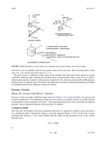
13.2.2 THERMOELASTICITY IN A ROD
Consider a rod that is built into a large, rigid, nonconducting temperature reservoir

at x = 0. The force, f
0
, and heat flux, −q
0
, are prescribed at x = L. A single element
models the rod. Now,
(13.20)
The thermoelastic stiffness matrix becomes ΣΣ
ΣΣ
=
αλ
∫B
ν
T
dV → Σ =
αλ
A/2. The
governing equations are now
(13.21)
13.3 COMPRESSIBLE ELASTIC MEDIA
For a compressible elastic material, the isotropic stress S
kk
and the dilatational strain
E
kk
are related by S
kk
= 3
κ
E

kk
, in which the bulk modulus
κ
satisfies
κ
= E/[3(1 − 2
ν
)].
Clearly, as
ν
→ 1/2, the pressure, p = −S
kk
/3, needed to attain a finite compressive
volume strain (E
kk
< 0) becomes infinite. At the limit
ν
= 1/2, the material is said
to satisfy the internal constraint of incompressibility.
Consider the case of plane strain, in which E
zz
= 0. The tangent modulus matrix
D is readily found from
(13.22)
d
dt
T
1
2
1

2
12
22
zQz zQz
zQQz
K
TT
TT
T




=−
=− +
[]
=−θθθθ
uxt xtL Ext tL xtL
d
dx
tL( ,) ()/ , ( ,) ()/ , ()/ , ()/ .==−==
γγ θθ
T T
T
0
ρ
γγαλθ
ρ
θθαλγ
AL A

L
A
1
cAL
kA
L
A
e
3
3
11
2
00
˙˙
˙
˙
+− =
++ =−
E1
2
f
TT
q
0
0
S
S
S
E
E

E
xx
yy
zz
xx
yy
zz












=
+−
−−+
()
−+
()
−
−

























E
110
11 0
0012
2
2
()( )
.
112

νν
ννν
νν ν
ν
0749_Frame_C13 Page 177 Wednesday, February 19, 2003 5:19 PM
© 2003 by CRC CRC Press LLC
178 Finite Element Analysis: Thermomechanics of Solids
Clearly, D becomes unbounded as
ν
→ 1/2. Furthermore, suppose that for a
material to be nearly incompressible,
ν
is estimated as .495, while the correct value
is .49. It might be supposed that the estimated value is a good approximation for
the correct value. However, for the correct value, (1 − 2
ν
)
−1
= 50. For the estimated
value, (1 − 2
ν
)
−1
= 100, implying 100 percent error!
13.4 INCOMPRESSIBLE ELASTIC MEDIA
In an incompressible material, a pressure field arises that serves to enforce the
constraint. Since the trace of the strains vanishes everywhere, the strains are not
sufficient to determine the stresses. However, the strains together with the pressure
are sufficient. In FEA, a general interpolation model is used at the outset for the
displacement field. The Principle of Virtual Work is now expressed in terms of

the displacements and pressure, and an adjoining equation is introduced to enforce
the constraint a posteriori. The pressure can be shown to serve as a Lagrange
multiplier, and the displacement vector and the pressure are varied independently.
In incompressible materials, to preserve finite stresses, we suppose that the
second Lame coefficient satisfies
λ
→ ∞ as tr(E) → 0 in such a way that the product
is an indeterminate quantity denoted by p:
(13.23)
The Lame form of the constitutive relations becomes
(13.24)
together with the incompressibility constraint E
ij
δ
ij
= 0. There now are two inde-
pendent principal strains and the pressure with which to determine the three principal
stresses.
In a compressible elastic material, the strain-energy function w satisfies S
ij
= ,
and the domain term in the Principle of Virtual Work can be rewritten as ∫
δ
E
ij
S
ij
dV =
∫
δ

wdV. The elastic-strain energy is given by w =
µ
E
ij
E
ij
+ . For reasons
explained shortly, we introduce the augmented strain-energy function
(13.25)
and assume the variational principle
(13.26)
λ
tr p() .E →−
SEp
ij ij ij
=−2
µδ
,
∂
∂
w
E
ij
λ
2
E
k
k
2
′

=−wEEpE
ij ij
kk
µ
δδρ δ
′
+=
∫∫ ∫
wdV dV dS
o
T
oo
T
o
uu u
˙˙
.
ττ
0749_Frame_C13 Page 178 Wednesday, February 19, 2003 5:19 PM
© 2003 by CRC CRC Press LLC
Thermal, Thermoelastic, and Incompressible Media 179
Now, considering u and p to vary independently, the integrand of the first term
becomes
δ
w′ =
δ
E
ij
[2
µ

E
ij
− p
δ
ij
] −
δ
pE
kk
, furnishing two variational relations:
(13.27)
The first relation is recognized as the Principle of Virtual Work, and the second
equation serves to enforce the internal constraint of incompressibility.
We now introduce the interpolation models:
(13.28)
Substitution serves to derive that
(13.29)
Assuming that these equations apply at the global level, use of state form
furnishes
(13.30)
The second matrix is antisymmetric. Furthermore, the system exhibits marginal
asymptotic stability; namely, if f(t) = 0 while (0), γγ
γγ
(0), and ππ
ππ
(0) do not all vanish,
then
(13.31)
δδρδ
δ

E S dV u u dV dS
pE dV
ij ij o
T
oo
T
o
kk
∫∫ ∫
∫
+=
=
˙˙
u
ττ
(a)
(b)
0
0
uN Bx
bxx
==
==
TT
kk
TT
tt
Extp t
((
(()()

xg g
gxp
) ( ) ) ( )
) ( ) ( )
e
MK f
˙˙
() () ()
,()
γ
ttt
dV t
o
+−=
==
∫
γγΣΣππ
ΣΣξξΣΣγγb
TT
0
M00
0K0
000
0K
K0 0
00
f
0
0
TT T T



























+
−
−



























=





d
dt
t
t
t
t
t
t
t
˙
()
˙
()
()
˙
()
()
()
()γγ
γγ
ππ
ΣΣ
ΣΣ
γγ
γγ
ππ









.
˙
γγ
d
dt
ttt
t
t
t
1
2
0(
˙
() () ())
˙
()
()
()
γγγγππ
γγ
γγ
ππ
TTT
TT
M00
0K0

000



































=
0749_Frame_C13 Page 179 Wednesday, February 19, 2003 5:19 PM
© 2003 by CRC CRC Press LLC
180 Finite Element Analysis: Thermomechanics of Solids
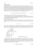
13.5 EXERCISES
1. Find the exact solution for a circular rod of length L, radius r, mass density
ρ
, specific heat c
e
, conductivity k, and cross-sectional area A =
π
r
2
. The
initial temperature is T
0
, and the rod is built into a large wall at fixed
temperature T
0
(see figure below). However, at time t = 0, the temperature
T
1
is imposed at x = L. Compare the exact solution to the one- and two-
element solutions. Note that for a one-element model,
2. State the equations of a thermoelastic rod, and put the equations for the

thermoelastic behavior of a rod in state form.
3. Put the following equations in state form, apply the trapezoidal rule, and
triangularize the ensuing dynamic stiffness matrix, assuming that the tri-
angular factors of M and K are known.
4. In an element of an incompressible square rod of cross-sectional area A,
it is necessary to consider the displacements v and w. Suppose the length
is L, the lateral dimension is Y, and the interpolation models are linear for
the displacements (u linear in x, with v,w linear in y) and constant for the
pressure. Show that the finite-element equation assumes the form
and that this implies that 3
µ
= f (which can also be shown by an a
priori argument).
kA
L
Lt
cAL
Lt qL
e
θ
ρ
θ
(,)
˙
(,) ().+=−
3
T
0
T
1

,t>0
r
L
M K f, 0
T
˙˙
.γγγγΣΣππΣΣγγ+−= =
20
04 2
20
0
0
2
µ
µ
AL A
AL Y AL Y
AALY
uL
vY
p
f/
//
/
−
−























=










()

()
uL
L
()
0749_Frame_C13 Page 180 Wednesday, February 19, 2003 5:19 PM
© 2003 by CRC CRC Press LLC