Finite Element Analysis - Thermomechanics of Solids Part 15 pot

195

Introduction to Contact
Problems

15.1 INTRODUCTION: THE GAP

In many practical problems, the information required to develop a finite-element
model, for example, the geometry of a member and the properties of its constituent
materials, can be determined with little uncertainty or ambiguity. However, often
the loads experienced by the member are not so clear. This is especially true if loads
are transmitted to the member along an interface with a second member. This class
of problems is called contact problems, and they are arguably the most common
boundary conditions encountered in practical problems. The finite-element commu-
nity has devoted, and continues to devote, a great deal of effort to this complex
problem, leading to gap and interface elements for contact. Here, we introduce gap
elements.
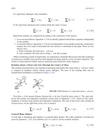
First, consider the three-spring configuration in Figure 15.1. All springs are of
stiffness

k

. Springs

A

and

C

extend from the top plate, called the

contactor

, to the
bottom plate, called the

target

. The bottom of spring

B

is initially remote from the
target by a gap

g

. The exact stiffness of this configuration is
(15.1)
From the viewpoint of the finite-element method, Figure 15.1 poses the following
difficulty. If a node is set at the lowest point on spring

B

and at the point directly

FIGURE 15.1

Simple contact problem.

15
k
kg
kg
c
=
<
≥





2
3


δ
δ
.
contactor
P
ABC
δ
kk k
g
target

0749_Frame_C15 Page 195 Wednesday, February 19, 2003 5:20 PM
© 2003 by CRC CRC Press LLC

196

Finite Element Analysis: Thermomechanics of Solids

below it on the target, these nodes are not initially connected, but are later connected
in the physical problem. Furthermore, it is necessary to satisfy the

nonpenetration
constraint

whereby the middle spring does not move through the target. If the nodes
are considered unconnected in the finite-element model, there is nothing to enforce
the nonpenetration constraint. If, however, the nodes are considered connected, the
stiffness is artificially high.
This difficulty is overcome in an approximate sense by a bilinear contact element.
In particular, we introduce a new spring,

k

g

, as shown in Figure 15.2.
The stiffness of the middle spring (

B

in series with the contact spring) is now
denoted as

k

m

, and
(15.2)
It is desirable for the middle spring to be soft when the gap is open (

g

>

δ

) and
to be stiff when the gap is closed (

g



≤



δ

):
(15.3)
Elementary algebra serves to demonstrate that

(15.4)
Consequently, the model with the contact is too stiff by 0.5% when the gap
is open, and too soft by 0.33% when the gap is closed (contact). One conclusion
that can be drawn from this example is that the stiffness of the gap element should
be related to the stiffnesses of the contactor and target in the vicinity of the contact
point.

FIGURE 15.2

Spring representing contact element.
contactor
target
P
AB
C
δ
kk k
k
g
k
kk
m
g
=+









−
11
1
.
k
kg
kg
g
=
>
≤





/100

δ
δ
100 .
k
kkg
kkg
c
≈
+>
+≤






2001
2099
.



δ
δ

0749_Frame_C15 Page 196 Wednesday, February 19, 2003 5:20 PM
© 2003 by CRC CRC Press LLC

Introduction to Contact Problems

197

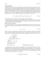
15.2 POINT-TO-POINT CONTACT

Generally, it is not known what points will come into contact, and there is no
guarantee that target nodes will come into contact with foundation nodes. The gap
elements can be used to account for the unknown contact area, as follows. Figure 15.3
shows a contactor and a target, on which are indicated candidate contact areas, d

S

c

and d

S

t

, containing nodes c1, c2,… ,cn, t1, t2,… ,tn. The candidate contact areas
must contain all points for which there is a possibility of establishing contact.
The gap (i.e., the distance in the undeformed configuration) from the

i

th

node of
the contactor to the

j

th



node of the target is denoted by

g

ij

. (For the purpose of this
discussion, the gap is constant, i.e., not updated.) In point-to-point contact, the

i

th

node on the contactor is connected to each node of the target by a spring with a
bilinear stiffness. (Clearly, this element may miss the edge of the contact zone when
it does not occur at a node.) It follows that each node of the target is connected by
a spring to each of the nodes on the contactor. The angle between the spring and
the normal at the contactor node is

α

ij

, while the angle between the spring and the
normal to the target is

α

ji

. Under load, the

i

th

contactor node experiences displacement

u

ij

in the direction of the

j

th

target node, and the

j

th

target node experiences displace-
ment

u

ji

. For example, the spring connecting the

i

th



contactor node with the

j

th

target
node has stiffness

k

ij

, given by
(15.5)
in which

δ

ij



=

u

ij



+



u

ji

is the relative displacement. The force in the spring connecting
the

i

th

contactor node and

j

th

target node is

f

ij



=



k

ij

(

g

ij

)

δ

ij

. The total normal force
experienced by the

i

th

contactor node is

f

i



=



∑

j



f

ij

cos(

α

ij

).

FIGURE 15.3

Point-to-point contact.
k
kg
kg
ij
ijlower
ij ij
ijupper ij ij
=
<
≥







δ
δ
,
candidate contactor contact surface
candidate target contact surface

dS
c
dS
t
c1
t1
t2
t3
c2
c3
α
31
k(g
31
)

0749_Frame_C15 Page 197 Wednesday, February 19, 2003 5:20 PM
© 2003 by CRC CRC Press LLC

198

Finite Element Analysis: Thermomechanics of Solids

As an example of how the spring stiffness might depend upon the gap, consider
the function
(15.6)
where

γ

,

α

, and

ε

are positive parameters selected as follows. When

g

ij



−



δ

ij

−



γ

>

0,

k

ij

attains the lower-shelf value,

k

0

ε

,



and we assume that

ε



<<

1. If

g

ij



−



δ

ij

−



γ



<

0,

k

ij

approaches the upper-shelf value,

k

0

(1

−



ε

). We choose

γ

to be a small value to
attain a narrow transition range from the lower- to the upper-shelf values. In the
range 0

<



g

ij



−



δ

ij



<



γ

, there is a rapid but continuous transition from the lower-shelf
(soft) value to the upper-shelf (stiff) value. If we now choose

α

such that

αγ

=

1,

k

ij

becomes

k

0

/2,



when the gap closes (

g

ij



=

δ

ij

). The spring characteristic is illustrated
in Figure 15.4.
The total normal force on a contactor node is the sum of the individual contact-
element forces, namely
(15.7)
Clearly, significant forces are exerted only by the contact elements that are
“closed.”

FIGURE 15.4

Illustration of a gap-stiffness function.
kg
kgg
ij ij ij
ij ij ij ij
()
()tan()(),
−
=+− −−−−−

















−
δ
εε
π
α
δγ δγ
0
12
12
2
2
fkg
tj ij ij ij ij ij
i
N
c
=−
∑
( ) cos( ).
δδ α

k
ij
k
0
/2
k
0
ε
k
0
ε
k
0
δ
ij
–g
ij
0749_Frame_C15 Page 198 Wednesday, February 19, 2003 5:20 PM
© 2003 by CRC CRC Press LLC
Introduction to Contact Problems 199
15.3 POINT-TO-SURFACE CONTACT
We now briefly consider point-to-surface contact, illustrated in Figure 15.5 using a
triangular element. Here, target node t3 is connected via a triangular element to
contactor nodes c1 and c2. The stiffness matrix of the element is written as k([g
1
−
δ
1
],
[g

2
−
δ
2
]) , in which g
1
−
δ
1
is the gap between nodes t1 and c1, and is the
geometric part of the stiffness matrix of a triangular elastic element. The stiffness
matrix of the element can be made a function of both gaps. Total force normal to
the target node is the sum of the forces exerted by the contact elements on the
candidate contactor nodes.
In some finite-element codes, the foregoing scheme is used to approximate the
tangential force in the case of friction. Namely, an “elastic-friction” force is assumed
in which the tangential tractions are assumed proportional to the normal traction
through a friction coefficient. This model does not appear to consider sliding and
can be considered a bonded contact. Advanced models address sliding contact and
incorporate friction laws not based on the Coulomb model.
15.4 EXERCISES
1. Consider a finite-element model for a set of springs, illustrated in the
following figure. A load moves the plate on the left toward the fixed plate
on the right.
What is the load-deflection curve of the configuration?
For a finite-element model, an additional bilinear spring is supplied, as
shown. What is the load-deflection curve of the finite-element model?
Identify a k
g
value for which the load-deflection behavior of the finite-

element model is close to the actual configuration.
Why is the new spring needed in the finite-element model?
FIGURE 15.5 Element for point-to-surface contact.
candidate target contact surface
candidate contactor contact surface
element connecting node
t3 with nodes c1 and c2
dS
t
dS
c
t2
t1
c1
c2
c3
t3
ˆ
K
ˆ
K
0749_Frame_C15 Page 199 Wednesday, February 19, 2003 5:20 PM
© 2003 by CRC CRC Press LLC
200 Finite Element Analysis: Thermomechanics of Solids
2. Suppose a contact element is added in the previous problem, in which the
stiffness (spring rate) satisfies
Suppose
αγ
= 1, k
L

= k/100, and k
u
= 100k. Compute the stiffness k for
the configuration as a function of the deflection
δ
.
F
H
L
k
k
k
k
k
kg
kgg
ij ij
ij ij ij ij
()
()tan()().
−
=+− −−−−−

















−
δ
εε
π
α
δγ δγ
0
12
12
2
2
0749_Frame_C15 Page 200 Wednesday, February 19, 2003 5:20 PM
© 2003 by CRC CRC Press LLC