Illustrated Sourcebook of Mechanical Components Part 9 pps
Bạn đang xem bản rút gọn của tài liệu. Xem và tải ngay bản đầy đủ của tài liệu tại đây (4.47 MB, 53 trang )
accurate specifications he has made for the cam profile.
The theory
of
envelopes has not been employed to
any extent in cam design-yet it is a powerful analytical
tool. The theory is illus:rated here and then applied to
the development of profile and cutter-coordinate equa-
tions for the six major types
of
cams:
Flat-face follower cams
0
Swinging in-line follower
Swinging off-set follower
Translating follower
Translating follower
Translating off-set follower
0
Swinging follower
Roller-follower cams
The design equations for these cams (the profile and
cutter-coordinate equations) are in a form that accepts
any profile curve-such as the cycloidal or harmonic
curve-or any other desired input-output relationship.
The cutter-coordinate equations are
not
a simple varia-
tion of the profile equations, because the normal fine
at the point of tangency of the cutter and the profile
does not continually pass through the cam center. We
had need for accurate cutter equations in the case
of
a
swinging flat-face follower cam. The search for the
solution led
us
to employ the theory of envelopes.
A
detailed problem of this case is included to illustrate the
use
of
the design equations which, in our application,
provided coordinates for cutting cams to a production
tolerance of
&0.0002
in. from point to point, and
0.002-in. total over-all deviation per cam cycle.
The question will come up whether computers are
necessary in solving the design equations. Computers
are desirable, and there are many outside services avail-
able. Calculations by hand or with
a
desk calculator
will be time consuming. In many applications, however,
the manual methods are worth while when judged by
the accuracy obtainable. The designer will undoubtedly
develop his own short cuts when applying the manual
methods.
Application
to
visual grinding
The design equations offered here can also be put to
good advantage in visual grinding. Magnification
is
limited by the definition of the work blank projected on
the glass screen. On a particular visual grinder, the
definition is good at a magnification
of
30X,
although
provision is made for
50X.
Using Mylar drawing film
for the profile, which is to be ked to the ground-glass
screen, a
30X
drawing
or
chart of portions of the cam
profile can be made. Best results are obtained by
locating the coordinate axis zero near the curve segment
being drawn and by increasing the number
of
calculated
points in critical regions to
YZ
or
%-deg increments for
greater accuracy. (Interpolation between points specified
in 2-deg intervals by means of a French curve, for
example, suffers in accuracy.) This procedure facilitates
checking
a
cam with a fixture employing
a
roller, be-
cause the position of the roller follower can be specified
simultaneously with the profile point coordinates.
The real limitation in visual grinding
is
the size of
ground-glass field and the limited scope of blank profile
which can be viewed at one time. If
30X
is the magnifi-
cation
for
good definition, and the screen is
18
in.,
the maximum cam profile which can be viewed at one
time is
18/30
=
0.60
in.
If
the layout is drawn
30
times size and
a
draftsman can measure
rtO.010
in., the
error in drawing the chart is
0.010/30
=
+0.0003
in.
In addition, the coordination of chart with
cam
blank,
Cams
18-19
IY
I
V”t1
X
f
mvelope
kc-‘
y=-l
IS
.
.
LINEARLY
MOVING
CIRCLES
The theory of envelopes is a topic in calculus not
always taught in college courses. It is illustrated here
by two examples, before we proceed to apply to it cam
design.
The envelope can be defined this way: If each member
of
an infinite family
of
curves is tangent to a certain
curve, and if at each point
of
this curve at least one
member
of
the family
is
tangent, the curve is either
a
part or the whole of the envelope
of
the family.
Linearly moving circle
equation
As
the first example of envelope theory, consider the
(x
-
cy
+
(y)Z
-
1
=
0
(1)
This represents a circle of radius
1
located with its
center at
x
=
c,
y
=
0.
As
c
is varied, a series of circles
are determined-the family of circles governed by Eq
1
and illustrated in Fig
1A.
Eq
1
can be rewritten
f(x,
Yt
c)
=
0
(2)
It is shown in calculus that the slope of any member
of the family of Eq
2
is
This may be written
(4)
(5)
This slope relation holds true for any member of the
family. If another curve (the envelope) is tangent
to
the member qf the family at a single point,
its
slope
likewise satisfies Eq
5.
18-20
1B
.
.
SHELL
TRAJECTORY IC
. .
PARABOLIC ENVELOPE
OF
TRAJECTORIES
It is also shown in calculus that the total dzerential
of
Eq
2
is
or
df
dx
df
dy
af
__I
+ +-=o
dx
dc by
dc
dc
From Eq
5
and
6,
the general equation for the envelope is
(7)
The envelope may be determined by eliminating the
parameter
c
in
Eq
7
or by obtaining
x
and
y
as func-
tions
of
c.
(The point having the coordinates at
x
and
y
is a point on the envelope, and the entire envelope
can be obtained by varying
c.)
Returning to Eq
1
and applying Eq
7
gives
=
2(x
-
c)
(-1)
+
0
-
0
=
0
Therefore
x
=
c.
Substituting this into
Eq
1
gives
y
=
el.
Thus the lines
y
=
+1
and
y
=
-1
are the
envelopes of the family
of
Eq
3.
This,
of course,
is
evident by inspection
of
Fig
1.
Shell
trajectories
As
a second example
of
envelope theory, consider the
envelope of all possible trajectories (the range envelope)
of
a gun emplacement.
If
the gun can be fired at any
angle
a
in a vertical plane with a muzzle velocity
v,,
Fig
lB,
what is the envelope which gives the maximum
range in any direction in the given vertical plane?
Air
resistance
is
neglected.
The equation
of
the trajectory
is
(8)
9x2
y
=
x
tan
a
-
-
(1
+
tan2
a)
2v,2
where
vo
=
muzzle
velocity
t
=
time
g
=
gravitational constant
Eq
8
is
derived
as
follows:
y
=
vo
sin
at
-
$gt2
where
t=-=2
X
v,
vo
cos
a
Substituting this value of
t
into Eq
9
gives
(9)
which can be readily put in the form
of
Eq
8.
the equation:
Rewriting Eq
8
so
that all factors are on one side
of
9x2
(1
+
tan2
a)
-
y
=
0
(12)
2v.
f(x,y,a)
=
x
tan
a,-
Thus
Solving Eq
13
for tan
a
gives
V2
tan
a
=
-
gx
Eliminating the parameter
a
by substituting this value
of
tan
a
into Eq
8
yields the envelope
of
the useful
range of the gun,
v2
9x2
y=2g-2U,2
which
is
a parabola, pictured
in
Fig
1C.
SYMBOLS
b
=
y-intercept of straight line
c
=
linear-distance parameter
e
=
offset of flat-face or roller follower
f
=
function notation
g
=
gravitational constant
J
=
[(rb
+
rf)2
-
e21112
L
=
lift of follower
m
=
general slope of straight line
r,
=
distance between pivot point of swing-
ing follower and cam center
Tb
=
radius of base circle of cam
rc
=
radius of cutter
R,
=
radius vector from cam center to cut-
ter center. Employed in conjunction
with
w
H
=
Tb
+
Tj
+L
ni=+-e+e
N=~-+-P
rj
=
radius
of
roller follower
rT
=
length of roller-follower arm
vo
=
initial (muzzle) velocity
t
=
time
x,
y
=
rectangular coordinates of cam profile,
or
of circle
or
parabola in examples on
envelope theory
xc,
yc
=
cutter coordinates to produce cam
profile
_-
a
-
total derivative with respect to x
dx
a
-
partial derivative with respect to
x
ax
a
=
angle of muzzle inclination in trajec-
tory problem; also angle between
x-axis and tangent to cutter contact
point
p
=
maximum lift angle for a particular
curvesegment
=
e,,,
w
=
angular displacement of cutter center,
referenced to zero
at
start of cam pro-
file rise. Employed
in
conjunction
with
R,.
B
=
angular displacement
of
cutter, ref-
erenced to x-axis, with the cam
considered stationary
(for
specifying
polar cutter coordinates);
e
=
tan-1
(yc/xc); also
e
=
w
when rise begins
at
x-axis as in Fig.
7.
e
=
cam angle of rotation
+
=
angular rotation or lift of the follower,
usually specified
in
terms
of
e
\E
=
angle between initial position
of
face
of swinging follower, and line joining
center
of
cam and pivot point
of
fol-
lower (a constant)
X
=
maximum displacement angle of fol-
lower arm
Cams
18-2
1
the condition of the machine, and the operator’s degree
of
skill
all add some error. In a particular segment,
the operator can grind
r+0.0003
in., but when the chart
and work piece are moved to the next profile segment
they must be properly coordinated to take advantage
of
the grinder’s skill and
to
prevent discontinuities that can
affect seriously the dynamic characteristics of the cam.
FLAT-FACE
FOLLOWERS
The theory of envelopes is now applied to finding
the design equations for cams with flat-face followers.
In general:
1
)
Choose a convenient coordinate system-both rec-
tangular and polar coordinates are given here.
2.
Write the general equation of the envelope, involv-
ing one variable parameter.
3)
Differentiate this equation with respect to the vari-
able parameter and equate it to zero. The total derivative
of the variable usually suffices (in place
of
the partial
derivative).
4)
Solve simultaneously the equations of steps
2
and
3
either to eliminate the parameter or to obtain the
coordinates of the envelope as functions of the parameter.
5)
Vary the parameter throughout the range
of
inter-
est to generate the entire cam profile.
Flat-face
in-line
swinging
follower
Flat-face swinging-follower cams are of the in-line
type, Fig
2,
if the face, when extended, passes through
the pivot point. The initial position of the follower
before lift starts
is
designated by angle
+.
This angle
is
a constant and can be computed from the equation
where
r
=
distance between cam center and pivot point
measured along x-axis
rb
=
radius of base circle of cam
The angular rotation
or
“lift” of the follower,
4,
is
the output motion.
It
is
usually specified as
a
function
of the cam angle of rotation,
0.
Thus
0
is the inde-
pendent variable and
4
the dependent variable.
A
well-known analytical technique
is
to assume the
cam
is
stationary and the follower moving around it.
Varying
0
and
4
and maintaining
I#
constant produces
a family of straight lines that can be represented as a
function of
x,
y,
8,
4.
Since
4
is in turn a function
of
e,
essentially there
is
f(x,Y,e>
=
0
(15)
This is the form of Eq
2.
Thus to obtain the envelope
of this family, which is the required cam profile, on::
solves simultaneously
Eq
15,
and
(16)
The first step
is
to
write the general form of the equa-
tion of the family. We begin with
y=mx+b
(17)
18-22
Where
b
is the y-intercept and
m
the slope. In this case,
m
is
equal to
m=-tan(+-
e+*)
(18)
Hence
Also
x
=
ra
COS
e
y
=
r,
sin
0
Solving for
b
results in
b
=
r,[sin
e
+
cos
e
tan
(4
-
0
+
*)I
(20)
Therefore
f(x,y,e)
=
Y
+
tan
(4
-
e
+
\E)
(X
-
r,
cos
e)
-
ra
sin
e
=
0
(21)
This equation
is
in the form of Eq
15.
It is now dif-
ferentiated with respect to
8:
$'-
=
tan
(4
-
e
+
q)ra
sin
e
+
dB
(z
-
r,
cos
B)[sec2
(4
-
0
+
q)]
For simplification
in
notation, let
~=d-e+q
The
rectanguiar coordinates
of
a
point
on
the
cam
profile
corresponding to
a
specific angle of cam rotation,
8,
are then obtained by solving Eq
21
and
22
simultane-
ously. The coordinates are
COS
(e
+
M)
COS
M
z
=
r,
COS
e
+
__-
d4
1
dB
L
-I
COS
(e
+
M)
cos
M
_
Cl4
1
d0
L
I
As
mentioned previously the desired lift equation,
Q,
is
usually known in terms
of
0.
For
example, in a
computer
a
cam must produce an input-output relation-
ship
of
Q
=
28".
In other words, when
6'
rotates
1
deg,
Q
rotates
2
deg; when
8
rotates
2
deg,
4
rotates
8
deg,
etc. Then
4
=
282
and
2
.
.
Flat-face swinging-follower cam
with
line
of
follower face extending through
pivot point.
Offsef
follower faces
r+e
A
Fol/ower
pivof
3
.
.
Two
types
of offset
flat-face follower.
yc
(cutter
coaro?nafesj
Cam
center
Norma/
fhrough
points
4
.
.
Cutter coordinates
for
flat-face swinging followcr.
Substituting the value of
C$
into the equation
for
m,
and the value of d4/dO into Eq
23
and
24
gives
x
and
y
in terms of
8.
Where the lift equation must also meet certain velocity
and acceleration requirements (as is the more common
case), portions of analytical curves in terms of
4,
such as
the cycloidal
or
harmonic curves, must be used and
matched with each other.
A
detailed cam design problem
of an actual application is given later to illustrate this
technique.
Offset swinging follower
The profile coordinates for
a
swinging flat-faced fol-
lower cam
in
which the follower face
is
not in line
with the follower pivot, Fig
3,
are
'Os
(e
+
M,
dd
-
cosM
I
+
e
sinM (25)
L
'Os
(e
M,
sin
M
+
e
COS
M
(26)
1
L
-I
where
e
=
the offset distance between a line through
the cam pivot and the follower face. Distance
e
is con-
sidered positive or negative, depending on the configura-
tion. In other words, the effect of
e
in
Eq
25
and
26
is to increase or decrease the size of the in-line follower
cam. When
e
=
0,
Eq
25
and
26
simplify to
Eq
23
and
24.
Cutter coordinates
For cam manufacture, the location of the milling
cutter or grinding wheel must be specified in rectangular
or polar coordinates-usually the latter.
The rectangular cutter coordinates for the
in-line
swinging follower,
Fig
4,
are
x.
=
x
+
rc
sin
M
y,
=
y
+
rc
cos
M
(27)
(28)
where
x,
y
=
profile coordinates
(Eq
23 and 24)
I
rc
=
radius
of
cutter
The
polar
coordinates
are
R,
=
(x2
+
yc2)1'2
(29)
(30)
w
=
90"
-
(\E
+
E)
where
E=
angular displacement of the cutter with respect
to the
x
axis, and with the cam stationary.
O=
angular displacement of the cutter center refer-
enced to zero at the start of the cam profile rise, for cam
specification purposes and convenience
in
machining.
The angles,
0,
and the corresponding distances,
R,,
are
subject to adjustment to
bring
these values
to
even
angles for convenience of machining.
This
will be illus-
trated later in the cam design example.
Cams
18-23
r
Cufter
5
. .
Radial
cam
with flat-face follower.
For offset swinging follower, the rectangular
coordi-
nates of the cutter are
x.
=
x
+
rc
sin
M
yo
=
y
+
re
cos
M
(32)
(33)
and the
polar
cutter coordinates are
R,
=
(x?
+
~?)l'z
(34)
Flat-face translating follower
The follower of this type of flat-face cam moves
radially, Fig
5.
The general equation of the family of
lines forming the envelope is
where
y=m+b
m
=
cos
8
L
=
lift
of follower
x
=
(rb
+
L)
cos
e
y
=
(rb
+
L)
sin
e
b
=
(rb
+
L)/sin
e
Hence
Therefore
f(x,y,e)
=
y
sin
0
+
x
cos
e
-
(rb
+
L)
=
0
(37)
and
dL
df
-
y
cos
e
-
x
sin
e
-
-
=
0
d0
de
(38)
18-24
,-
Roller
follower
6
.
.
Positive-action cam
with
double
envelope.
The profile coordinates
are
(by solving simultaneously
Eq
37
and
38):
(39)
dL
d0
2
=
(rb
+
L)
cos
0
-
-
sin
0
(40)
dL
d0
y
=
(rb
+
L)
sin
0
+
__
cos
e
where
L
is usually given in terms
of
the cam angle
0
(similar to
4
for the swinging follower).
The rectangular coordinates are
zc
=
2
+
rc
cos
0
yc
=
y
+
rE
sin
0
(41)
(42)
Polar coordinates
of
profile points
are obtained by
squaring and adding Eq
39
and
40:
Cutter
coordinates
in
polar
form
are obtained
by
squar-
ing and adding Eq
41
and
42.
Yo
w
=
tan-'
-
5.2
dL
d0
(EL
(rb
+
L
+
r,)
sin
0
+
-
cos
0
(Tb
+
1,
+
r,)
cos
0
-
sin
0
de
=
tan-'
(44)
7
.
.
Radial cam
with roller follower.
ROLLER FOLLOWERS
In determining the profile of a roller-follower cam by
envelope theory, two envelopes are mathematically pos-
sible-one the inner, profile envelope and the other an
outer envelope.
If
a positive-action cam is to be
constructed, Fig
6,
both envelopes are applicable, since
they constitute the slot in which the roller follower
would be constrained to move to give the desired output
motion.
The equations for three types of roller-follower cams
a,re derived below.
Translating
roller
follower
for this type of cam, Fig
7,
is
equal
to:
The radial distance,
H,
to the center of the follower
where
rf
=
radius
of
the
follower
roller
rb
=
base
circle
radius
L
=
lift
=
L(0)
The general equation
of
the envelope is
(Z
-
H
cos
+
(y
-
H
sin
e)z
-
rf2
=
0
(45)
The profile coordinates are
(by applying d/d0
=
0
and
solving for
y
and
x):
dL
Hsine cos0
+H-
d0
dL
]
d0
H
cos
0
+
-sin
0
(46)
dL
d0
Y=
Cams
18-25
and
x=Hcos8*
TI
dL
+
sin
8
-
;
cos
>]”’
(47)
H-cos
8
+
-
~~
sin
0
where
dL
dH
d8
d0
=
__
Here the plus-minus ambiguity may be resolved by
H
=
rb
+
rj
examining
8
=
0
when
x
=
rb.
At this point
and
x
=
rf
+
rb
*
rj
Only the negative sign
is
meaningful in the above
equation; thus the negative sign in Eq
47
establishes the
8
. .
Swinging
roller-followw cam.
inner envelope, and the plus sign the outer envelope,
which in this case is discarded.
The final equation
for
y
can be computed by sub-
stituting
Eq
47
into
46.
Rectangular coordinates
of
the
cutter
are
(48)
(49)
r
71
yE
=
y
+
2
(H
sin
8
-
y)
Polar
coordinates
of
the cutter are
R,
=
(x2
+
y,2)1’2
(50)
E
=
tan-’
E
(551)
XC
Swinging
roller
follower
equal to
This type of cam is illustrated in Fig
8.
Angle
$
is
The general equation of the family
is
[x
-
r,
cos
8
+
rr
cos
NI2
+
[y
-
r,
sin
0
+
r,
sin
N]2
-
=
0
(53)
where
N=8-+-*
The profile coordinates are
(by the method outlined
for the translating roller follower)
:
x
ra
sin
0
-
rr
(1
-
-$:-)
sin
N]
(54)
dl$
[
Y=
ra
cos
0
-
r,
(I
-
z)
cos
N
and
x
=
ra
cos
8
-
rr
cos
N
+
Referring to the
4
sign, the negative sign gives the
actual cam profile; the positive sign produces an outer
envelope. The equation for
y
can be computed by sub-
stituting Eq
55
into
54.
The rectangular cutter coordinates are:
9
.
.
08set
radial-roller
cum.
18-26
where
x,
and
y,,
the coordinates to the center
of
cutter,
are equal to
X~
=
T,
COS
e
-
r,
cos
N
yf
=
T,
sin
0
-
r,
sin
N
The polar cutter coordinates are
R,
=
(22
+
~2)"'
.
(58)
Translating offset roller follower
The
roller follower of this type of'cam, Fig
9,
moves
radially along a line that is offset from the cam center by
a distance
e.
[x
-
e
sin
0
-
(J
+
L)
cos
el2
+
The general equation of the envelope is
[y
+
e
cos
0
-
(J
+
L)
sin
e]'
-
rr'
=
0
(60)
where
J
=
[(rb
+
r,)?
-
e2]'/2
The profile coordinates are
(by applying d/dB
=
0,
and solving for
y
and
x)
:
(J+L)cos
e+(e+g)
sin
e
(6
1)
Y=
x
=
e
sin
0
+
(J
+
L)
cos
tJ
*
Tf-
Here again the negative sign of the plus-minus am-
biguity is physically correct.
The plus sign produces the
outer envelope.
Final equation for y can be obtained by substituting
Eq
62
into
61.
The rectangular cutter coordinates are
r,
Yc
=
Y
+
-
(Yr
-
Y)
Tf
(64)
where
xf
=
e
sin
e
+
(J
+
L)
cos
e
Yr
=
e
cos
e
+
(J
+
L)
sin
e
The polar cutter coordinates
are the
same
as Eqs 58 and
59.
NUMERICAL
EXAMPLE
The
design
specification
We have recently applied the cam equations to the de-
sign of a flat-faced swinging follower with face in line
with the follower pivot. The follower oscillates through
an output angle,
X,
with
a
dwell-rise-fall-dwell motion.
The angular displacement of the follower arm is speci-
fied by portions of curves which can be expressed as
mathematical functions of the angle of rotation of the
cam.
The specified angular motion
of
the arm consists
of a half-cycloidal rise from the dwell, followed by
half-harmonic rise and fall, and then by a half-cycloidal
return to the dwell,
as
shown
in
Fig
10.
Each region is
31.5 deg; the total cycle is completed in
126
deg.
Also included are the general shape of the follower
velocity and acceleration curves, which result from:
1)
the choice of curves,
2)
the stipulation that the cam
angle of rotation,
/3,
for each curve segment be equal,
and
3)
the stipulation that the angular velocity at the
matching points of the curves be the same for both
curves. The cam
is
to rotate
in
the counterclockwise
direction. It is to be specified by polar coordinates,
R,,
O,
in 1-deg increments.
Half
-
cyc/oid
Ha/f
-
hormomc
Hdf
-harmonic
Hdf
-
cycloid
rise
rise
fa//
foll
-126'
-94.5'
-63O
-315O
O%unferc/ockwise,
-B
(0)
($31.5')
(t63")
(t94.5O)
~t126a~~~Clockwise,
tB
10
.
.
Cam
design
problem,
illustrating cam layout,
top, phase diagrams, center, and displacement diagram.
Cams
18-27
The equations of angular displacement for the four
regions,
or
curve segments are
RSmg-region
1
(half-cycloid)
Rising-region
2
(half-harmonic)
@Z
=
ac
+
a~sin 90
X
-
(
O
*;)
Falling-region
3
(half-harmonic)
Falling-region
4
(half-cycloid)
44
=
ac
[;:(
1
-
-
-
-
sin 180"
X
-
;)]
where
A=
010
=
an
=
P=
8=
d
=
f(0)
=
Subscripts
:
maximum displacement angle of follower
arm
=
2.820,997,8 deg
half-cycloidal angle of displacement
of
follower
=
1.240,958,6 deg
half-harmonic angle of displacement of
follower
=
1.580,039,2 deg
e
maximum
=
maximum
lift
angle for
a
particular curve segment
=
-
31.5 deg
cam angle, degree
of
counterclockwise
rotation,
or
in a negative direction
instantaneous angle of displacement of
the follower
1
=
half-cycloidal, rising
2
=
half-harmonic,
rising
3
=
half-harmonic] falling
4
=
half-cycloidal, falling
Also
given are:
r.
=
3.2.5 in.
rb
=
1.1758 in.
9
=
21.209,369,3 deg
For
illustrative purposes, however, the computations
are rounded to four decimal places.
Solution
Eq
23
and
24
will give the
x
and
y
coordinates of
the profile. The derivative, d+/dO,
is
also
the angular
velocity
of
the follower.
The computations for locating the proEle when
0
=
-40
deg are presented below.
All
angles are in degrees:
3
=
1.2406
+
1.5800
=
1.8908 deg
=
-0.0718
M
=
4
-
e
+
\k
=
1.8909
-
(-40)
+
21.2094
=
63.1002 deg
From
Eq
23:
-
-
~0~(63.1002-40)~0~(63.1002)
(-0.718-1)
s_4o0=3.25 COS( -40)
+
1
=
1.2278 in.
Similarly, from Eq
24:
y
=
0.3983 in.
The cutter coordinates are obtained by means of Eq
27
through
31,
and
zc=z+rcsinM
=
1.2278
+
1.5
sin 63.1002
=
2.5655 in.
yc
=
y
+
rc
cos
M
=
1.0769 in.
R,
=
(z.,2
+
y.,2)1/z
=
[2.5655'
4-
1.07692]"2
=
2.7823 in.
=
tan-'
0796
=
22.7713 deg
2.5655
w
=
90
-
(9
+
E)
=
go
-
(21.2094
+
22.7713)
=
46.0193 deg
18-28
Cams and Gears Team
Up
-
in Programmed Motion
Pawls and ratchets are eliminated in this design, which
is
adaptable
to the smallest or largest requirements;
it
provides a multitude of
outputs
to
choose from at low
cest.
Theodore
Simpson
A new and extremely versatile
mechanism provides
a
programmed
rotary output motion simply and in-
expensively. It has been sought
widely for filling. weighing. cutting,
and drilling in automatic and vend-
ing machines.
The mechanism, which
uses
over-
lapping gears and cams (drawing be-
low),
is the brainchild
of
mechanical
designer Theodore Simpson
of
Nashua,
N.
H.
Based on a patented concept that
could be transformed into a number
of
configurations
,
PRIM
(Programmed Rotary Intermittent
Motion), as the mechanism is called,
satisfies the need for smaller devices
for
instrumentation without using
spring pawls or ratchets.
It
can be made small enough for
a
wristwatch or as large as required.
Versatile
output.
Simpson reports
the following major advantages:
Input and output motions are
on
a concentric axis.
*Any number
of
output motions
of varied degrees
of
motion
or
dwell
time per input revolution can be pro-
vided.
*Output motions and dwells are
variable during several consecutive
input revolutions.
*Multiple units can be assembled
on a single shaft to provide an al-
most limitless series
of
output mo-
tions and dwells.
*The output can dwell, then snap
around.
How
it
works.
The basic model
Basic intermittent-motion mechanism,
at
left
in
drawings,
goes
through
the rotation sequence
as
numbered
above.
Cams
18-29
(drawing, below left) repeats the
output pattern. which can be made
complex, during every revolution
of
the input.
Cutouts around the periphery
of
the cam give the number
of
motions.
degrees
of
motion, and dwell times
desired. Tooth sectors
in
the program
gear match the cam cutouts.
Simpson designed the locking levex
so
one
edge follows the cam aAd the
other edge engages or disengages,
locking or unlocking the idler gear
and output. Both program gear and
cam are lined
up.
tooth segments to
cam cutouts. and fixed to the input
shaft. The output gear rotates freely
on the same shaft, and an idler gear
meshes with both output gear and
segments
of
the program gear.
As the input shaft rotates, the
teeth
of
the program gear engage the
idler. Simultaneously, the cam
re-
leases the locking lever and allows
the idler to rotate freely, thus driv-
ing the output gear.
Reaching a dwell portion, the
teeth of the program gear disengage
from the idler, the cam kicks in the
lever to lock the idler, and the out-
put gear stops until the next program-
gear segment engages the idler.
Dwell time is determined by
the
space between the gear segments.
The number
of
output revolutions
does not have to
be
the same as the
number of input revolutions. An idler
of a different size would not affect
the output, but a cluster idler with a
matching output gear can increase or
decrease the degrees of motion to meet
design needs.
For example, a step-down cluster
with output gear to match could re-
duce motions to fractions
of
a de-
gree, or a step-up cluster with match-
ing output gear could increase motions
to several complete output revolutions.
Snap action.
A second cam and
a spring are used
in
the snap-action
version (drawing below). Here, the
cams have identical cutouts.
One cam is fixed to the input and
the other is lined up with and fixed
to the program gear. Each cam has a
pin in the proper position
to
retain
a spring; the pin of the input cam
extends through a slot in the pro-
gram gear cam that serves the func-
tion
of
a stop pin.
Both cams rotate with the input
shaft until a tooth of the program
gear engages the idler, which is
locked and stops the gear. At this
point, the program cam is in position
to release the lock, but misalignment
of
the peripheral cutouts prevents it
from doing
so.
As the input cam continues to
ro-
tate, it increases the torque
on
the
spring until both cam cutouts line
up.
This positioning unlocks the idler and
output, and the built-up spring torque
is suddenly released. It spins the pro-
gram gear with a snap as far as
the
stop pin allows; this action spins
the
output.
Although both cams are required
to release the locking lever and out-
put, the program cam alone
will
re-
lock the output-a feature
of
con-
venience and efficient use.
After snap action is complete and
the output is relocked, the program
gear and cam continue
to
rotate with
the input cam and shaft until they
are stopped again when a succeed-
ing tooth of the segmented program
gear engages the idler and starts
the
cycle over again.
Program gear
Spring
-@‘%I
1
2
3
Snapaction version,
with
a spring and with a second cam fixed
to
the program gear, works
as
shown in numbered sequence.
18-30
Minimum Cam Size
Whether for high-accuracy computers or commercial
screw machines-here’s your starting point for any
can design problem.
Preben
W.
Jensen
HE
best way to design
a
cam is
T
first
to
select
a
maximum pressure
angle-usually
30
deg for translat-
ing followers and
45
deg for swinging
followers-then lay
out
the cam pro-
file
to meet the other design require-
ments. This approach will ensure
a
minimum cam size.
But there are at least six types
of
profile curves in wide use today-
constant-velocity, parabolic, simple
harmonic, cycloidal,
3-4-5
polynomial,
and modified trapezoidal-and to de-
sign the cam to stay within a given
pressure angle for any given curve is a
time-consuming process. Add to this
the fact that the type
of
follower
employed also influences the design,
and you come up with a rather diffi-
cult design problem.
You
can avoid all tedious work by
turning to the unique design charts
presented here (Fig
5
to
10).
These
charts are based on
a
construction
method (Fig
1
to
4)
developed in
Germany by Karl Flocke back in
1931
and published by the German
VDI
as Research Report
345.
Flocke’s
method is practically unknown
in
this
country-it does not appear in any
Sym
bois
e
=
offset (eccent,ricit,y) of cam-follower center-
line with camshaft centerline, in.
Rb
=
base radius of cam, in.
Rf
=
roller radius, in.
R,,,
=
minimum radius to pitch curve, in.;
R,,
=
maximum radius
to
pitch curve, in.
y
=
linear displacement of follower, in.
y,,,
=
prescribed maximum cam stroke, in.
Lf
=
length of swinging follower arm, in.
R,,,
=
Rb
4-
Rf
a
=
pressure angle, deg-the angle between the
cam-follower centerline and the normal to
the cam surface
at
the point of roller contact
q~,
=
angle of oscillation of swinging follower,
deg
p
=
cam angle rotation, deg
7
=
slope
of
cam diagram, deg
published work.
It
is
repeated
here
because it is a general method applica-
ble to any type
of
cam curve
or
com-
bination
of
curves. With it you can
quickly determine the minimum cam
size and the amount
of
offset that
a
follower needs-but results may not
be accurate in that the points
of
max
pressure angle must be estimated.
The design charts, on the other
hand, are applicable only to the six
types
of
curves listed above. But they
are much quicker to use and provide
more accurate results.
Also
included in this article are
Offset
translating
roller
follower
Cams
18-3
1
0
3.
Location
of
cam
center
18-32
eight mec anisms for reducing the
pressure angle when the maximum per-
missible pressure angle must
be
ex-
ceeded
for
one reason or another.
Why
the emphasis on pressure angle?
Pressure angle is simply the angle
between the direction where the
fol-
lower wants to go and the direction
where .the cam wants to push it. Pres-
sure angles should be kept small
to
reduce side <&rusts on the follower.
But small pressure angles increase cam
size which in turn:
Increases the size of the maohine.
.Increases the number
of
precision
points and cam material
in
manufac-
turing.
Increases the circumferential speed
of
the cam which leads to unnecessary
vibrations in the machine.
Increases the cam inertia which
slows up starting and stopping times.
Translating followers
Flocke’s method
for
finding the
minimum cam size-in other words
e,
R,,.
and
R,,,
(see list
of
symbols)
-is as follows:
In
Fig
1
1.
Lay out the cam diagram (time-
displacement diagram) as the problem
requires. Type
of
curve to be em-
ployed-parabolic, harmonic, etc-
depends upon the requirements. Cam
rise is during portion
of
curve
AB;
cam return, during
CD.
2.
Choose points
of
maximum slope
during rise and return (points
PI
and
P2).
The maximum pressure angle
will occur near, or sometimes at, these
points.
3.
Measure slope angles
7,
and
r2.
4.
Measure the length,
L,
in inches
5.
Calculate
k:
corresponding to
360
deg.
L
2n
k=-
In Fig
2
1.
Lay out k and angles
r1,
7,.
This
locates points
Q,
and
QZ.
2.
Measure k(tan
rl)
and k(tan
7,).
.In Fig
3
1.
Lay out vertical line,
FG,
equal
to
total displacement,
ymar.
2.
Lay out from point
F,
the dis-
placements
y1
and
yz
(at points
P,
and
Pz).
This locates points
M
and
N.
3.
Lay out k(tan
rl)
to left of
M
to obtain point
E,.
Similarly k tan
TZ
to right from
N
locates
E,
(for
CCW rotation
of
cam).
4.
At points
El
and
E,
locate the
desired (usually maximum permis-
sible) pressure angles of points
P,
and
P,.
These angles are designated as
a,
and
a,.
5.
The lines define the limits
of
an area A. Any cam shaft center
chosen within this area will result in
pressure angles at points
PI
and
P,
which will be equal to or less than
the prescribed angles
a,
and
as.
If
the cam shaft center is chosen any-
where along Ray I, the-pressure angle
at
E,
will be exactly
a,
(and similarly
along Ray I1 for
a,).
Thus, if
0,,
the
intersection
of
these two rays, is
chosen as the cam center, the layout
will provide the desired pressure angles
for both rise and return.
6.
The construction results in an
offset roller follower whose eccen-
tricity,
e,
is measured directly on the
drawing. Radii R,,, and
R,,,
are also
measured directly on the drawing. The
actual cam shape
is
drawn
to
scale
in Fig
4.
Design charts
The above procedure, however, does
not ensure that the pressure angle is
not exceeded at some other point.
Only for some cases
of
parabolic
rno-
tion will the maximum pressure
angle
occur
at
the point
of
maximum slope.
Thus the same procedure has to be
repeated for numerous points during
the rise and return motions. The six
charts (Fig
5
to
10)
developed by
the author avoid the need for repeti-
tive construction. Also, for cases where
the cam size has already been chosen,
the charts provide the maximum pres-
sure angle during rise and return mo-
tions.
The scale of all the charts assumes
that the stroke
is
equal to one unit.
Hence, if
ymax
=
1
in. then the scales
can be read
off
directly in inches.
Design problem
All charts, Fig
5
to
10,
show con-
struction for the case where cam ro-
tation during cam rise and fall re-
spectively is
p1
=
25
deg and
@*
=
80
deg; total stroke,
ymar
=
2
in; max
\
5.
Simple
Harmonic
Motion
\
4
3
-2
-3
-4
-e
-+*++-+
,
i
L
Cams
18-33
\
/
I
I
\
.\
/
\
/
\
/
\
/
4
1:
I:
I\'[''
'?
,
,/'
,
+e
,
4
3
J
',
'
/
\1/
4
\
3
6.
Cycloidal
Motion
-5
60'50'
40'35'' 30" 25'
20"
-
7.
Chart for
3-4-5
Polynomial
-4
-e
+
pressure angle during rise,
a,
=
30
deg; during return,
a:.
=
30
deg. The
cam rotates counterclockwise (CCW)
.
Assume simple harmonic motion (Fig
5).
Construction
I.
Because rotation is CCW, go to
the left
of
center for the rise stroke,
and to the right for the return stroke,
as noted on the chart. Thus go to
the
p
=
25
deg curve and layout
angle
a,
=
30
deg
tangent
to the curve.
Lay out tangent to the
/3
=
80
deg
curve.
2.
The point where the two lines
intersect locates the cam shaft center
0,.
3.
Read down
to
the
e
scale
to
.+
0,
obtain the required eccentricity. Hence
e
=
(1.23)(2)
=
2.46
in. (multiply
by
2
because
ymu.
=
2
in.).
4.
Distance
0,F
is
RmI
To
obtain
its scale value, swing an arc
from
F
to
locate
0,.
Hence
R.,I.
=
(3.85)
(2)
=
7.7
in.
5.
Distance
0,G
=
R,,,
=
(4.83)
(2)
=
9.66
in.
All dimensions required to construct
the minimum cam size are now known.
You
can also determine what part
of
the stroke the maximum pressure
angle will occur at by noting the points
of
tangency
of
the
a,
and
ap
lines to
the 25-deg and 80-deg curves. Extend
these points horizontally to the
FG
line. Thus the max pressure angle
occurs
rk
of
the stroke upward during
rise, and
tQ
of the stroke downward
during return.
If
you want to know the pressure
angle, say at a point one quarter
of
the stroke during rise,
go
upward one
quarter
of
the distance from
F
to
G.
then to the left to intersect the
25
deg
curve. Connect this point
of
inter-
section to
0,.
The angle that this
new line makes with the vertical will
be the requested pressure angle.
For
parabolic cams
The procedure is slightly different
here (Fig
9).
The elongated curves
are pointed at the ends. Thus the lines
for
pressure angles
a,
and
us
are not
tangent to the curve
for
the numerical
18-34
\
/I
8.
Modified
Trapezoidal Curve
\
,I
CCWreturn
-
\
CCWrise
\-
\
\
1
9.
Parabolic
Motion
J-5
T
T
T
I
1
I
I
I
f
i
1
I
1
1
JO"
/5O
20"
C
W
return
LCW
rise
.IC
,/-
T"
10.
Constant
-
Velocity
Motion
./
-\,
q?'
T
'1'"
I
Cams
18-35
Type
of
cam
Max
radius,
Eccentricity,
R
max
e
I
Constant velocity
I
3.65
I
0.8
I
Parabolic motion
Simple harmonic motion
5.90
1.58
4.80 1.24
I
Cycloidal motion
I
5.90
1
1.58
I
3-4-5
Polynomial
Modified trapezoidal
Double harmonic motion 5.85
1.60
B
C
It.
Cam
diagram
m0::i
nr
12.
Slope
analysis
a,
13.
Location
of
conditions given (but in some cases
the lines may be).
For
constant
velocity cams
The elongated curves for this type
of
motion become vertical lines (Fig
10). Use the lower points of these
lines for laying out
a,
and
%,
as shown
by the dashed lines.
Comparison
of
cam
sizes
A
comparison of the required cam
sizes for the six types of cam con-
tours is given at the top
of
this page.
Note that t:ie constant-velocity curve
requires the smallest cam size.
Swinging followers
Cams with swinging followers re-
quire a construction technique similar
to
the Flocke method described previ-
Assume that a cam diagram
is
given
(Fig 11). Also known are the length
of follower arm,
L,,
and the angle of
arm oscillation during rise and fall,
+o.
The length of the circular arc through
which the roller follower swings must
be equal to
ymn.
in Fig
11.
(See p.
69
for an illustration of a swinging fol-
lower cam.)
The
construction technique, illus-
ously.
trated in Fig
11,
12
and
13,
is
as
follows:
1.
Divide the ordinate of the cam
diagram into equal parts (8 in this
case).
2. Select points along the divisions
and find the slope angles at the points.
The procedure is shown only for
points
P,
and
Pz,
but it should be
repeated for Other points.
3.
Calculate
k
=
L/(~T).
In
Fig
12, lay
off
k
and angles
T~
and
72.
Ob-
tain
k
(tan
7J
and
k
(tan
T~).
4.
In
Fig
13
lay
off
L,
(from
S
to
F)
and divide
4o
into
8
equal parts.
5.
Lay out
y1
and
y.
as shown (in
this case
yI
and
ys
are equal).
6.
If cam rotation is away from
pivot point
S
(counterclockwise in this
case) lay
off
ME,
=
k
tan
7,
to
the
left of point
M,
and
ME,
=
k
tan
7e
to the right of point
M.
(Reverse di-
rections for clockwise rotation of
cam,)
8.
Lay out
a,
and
a,
at
E,
and
Ell.
Repeat procedure for other points
as
shown. Now choose the lowest line
from both ends
to
obtain an area,
A,
which is the farthest area possible
from
F.
This results in Ray
f
and Ray
11.
If
a
cam shaft center is chosen
anywhere within this area, the maxi-
mum pressure angle will not be ex-
ceeded, either during rise or return.
9.
If
0,
is chosen, the maximum
pressure angles during rise will
OCCUI
at the middle of the stroke because
Ray
I
is determined from
E,,
which in
turn corresponds to the middle of the
stroke. Note that the maximum pres-
sure angle for the return stroke will
occur when the follower moves back
%
of the stroke because Ray
I1
origi-
nates from
a
point
%
of angle
&,
measured downward from the top.
18-36
t7n2
14.
Slidingcam
outpur
E
D
/npUt
15.
Stroke-
multiplying
mechanism
ff9
16.
Double-
faced cam
17.
Cam-and- rack
When the pressure angles are too
high to satisfy the design requirements,
and. it is undesirable to enlarge the
cam size, then certain devices can be
,:mployed to reduce the pressure
angles:
Sliding cam, Fig 14-This device is
used on a wire-forming machine. Cam
D
has a rather pointed shape because
of the special motion required for
twisting wires. The machine operates
at slow speeds, but the principle em-
ployed here
is
also applicable to high-
speed cams.
The original stroke desired is
(y,
+
yz)
but this results in a large
pressure angle. The stroke therefore
is reduced to
y,
on one side
of
the
cam, and a rise
of
y,
is added to the
other side. Flanges
B
are attached to
cam shaft
A.
Cam
D,
a rectangle with
the two cam ends (shaded), is shifted
upward as it cams
off
stationary roller
R.
during which the cam follower
E
is being cammed upward by the other
end of cam
D.
Stroke multiplying mechanism, Fig
15-This device is employed in power
presses. The opposing slots, one in a
fixed member
D
and the second in the
movable slide
E,
multiply the motion
of
the input slide
A
driven by the cam.
As
A
moves upward,
E
moves rapidly
to the right.
Double-faced cam, Fig 16
-
This
device doubles the stroke, hence re-
duces the pressure angles
to
one-half
their original values. Roller
R,
is sta-
tionary. When the cam rotates, its
bottom surface lifts itself on
R,,
while
its top surface adds an additional mo-
tion to the movable roller
R2.
The out-
put is driven linearly by roller
Rz
and
thus is approximately the sum of the
rise
of
both surfaces.
Cam-and-rack, Fig 17-This device
increases the throw of a lever. Cam
B
rotates around
A.
The roller follower
18.
Auxiliary cam system
travels at distances
yl,
during which
time gear segment
D
rolls on rack
E.
Thus the output stroke
of
lever
C
is
the sum
of
transmission and rotation
giving the magnified stroke
y.
Cut-out
cam, Fig 18-A rapid rise
and fall within
72
deg was desired.
This originally called for the cam
contour,
D,
but produced severe pres-
sure angles. The condition was im-
proved by providing an additional cam
C
which also rotates around the cam
center
A,
but at five times the speed
of cam
D
because
of
a
5:l
gearing
arrangement (not shown). The origi-
nal cam is now completely cut away
for the
72
deg (see surfaces
E).
The
desired motion, expanded over
360
deg
(since
72
x
5
=
360),
is now designed
into cam
C.
This results in the same
pressure angle as would occur if the
original cam rise occurred over
360
deg instead of
72
deg.
Cams
18-37
20.
Whit
worth
quick
-
re
turn
I
90"
21.
Drag
link
22.
Modification
of
original
cam
shape
v4
Desired
disp
facemen
f
90"
180'
270"
360'
Double-cam mechanism, Fig
19-
If you were to increase the cam speed
at the point of high-pressure angles,
and change the contour accordingly,
the pressure angle would be reduced.
The device in Fig
19
employs two cam
grooves to change the input speed
A
to the desired varying-speed output
in shaft
B.
Shaft
B
then becomes the
cam shaft to drive the actual cam (not
shown). If the cam grooves are cir-
cular about point
0
then the output
will be a constant velocity. Distance
OR
therefore is varied to provide the
desired variation in output.
Whitworth quick
return
mechanism,
Fig
20-This is a simpler way of
im-
parting a varying motion to the out-
put shaft
B.
However, the axes,
A
and
B,
are not colinear.
Drag link, Fig
21-This
is
another
simple device for varying the output
motion
of
shaft
D.
Shaft
A
rotates
with uniform speed. The construction
in Fig
22
shows how to modify the
original cam shape to take full ad-
vantage of the varying input motion
provided by shaft
D.
The construc-
tion steps are as follows (the desired
displacement curve is given at the top
of
Fig
22,
with the maximum pressure
angle designated as
7.J
:
1.
Plot the input vs output diagram
(0
vs
+)
for
the linkage illustrated in
Fig
21.
2.
Find the point with the smallest
slope,
P,.
3.
Pick any point
A
on
the tangent
to
P',
and measure the corresponding
angles to
P',
(32
deg and
20
deg).
4.
Go
20
deg to the right
of
P2
in
the cam diagram to locate
A'.
Also
locate
A
by going
32
deg to the right
of
P,
as shown. Point
A'
is on the
final cam shape. Repeat this pro-
cedure with more points until you ob-
tain the final curve. The pressure angle
at
P,
is thus reduced from
T~
to
7:.
18-38
Spherical
Cams:
Linking
Up
Shafts
European design
is
widely used abroad but little-known in
the
U.S.
Now a German engineering professor
is
telling the
story in this country, stirring much interest.
Anthony Honnavy
roblem: to transmit motion be-
P
tween two shafts in
a
machine
when, because
of
space limitations,
the shaft axes may intersect each
other.
One
answer is to use
a
spheri-
cal-cam mechanism, unfamiliar to
most American designers but used
in
Europe to provide many types
of
motion in agricultural. textile. and
printing machinery.
Recently, Prof.
W.
Meyer zur
Cappellen of the Institute of Tech-
nology, Aachen, Germany, visited
the
U.
S.
to show designers how
spherical-cam mechanisms work and
how to design and make them.
He
\
and his assistant kinematician at
Aachen,
Dr. G.
Dittrich, are in the
midst
of
experiments with complex
spherical-cam shapes and with the
problems
of
manufacturing them.
Fundamentals.
Key elements
of
spherical-cammechanism
(above
Fig.
1)
can be considered
as
being
posi-
i
,
Plane
ring
/
/
Input
cam
-
Spherical mechanism with radial follower
4
Cam mechanism with flat-faced follower
I
Radial roller follower shown on a sphere
1
Follower
,
Cams
18-39
Mechanism with radial roller follower shown on a sphere
Spring-
loaded
Input
cam
1
Spherical cam mechanism with radial follower
2
Cam mechanism with rocking roller follower
8-40
5
Hollowsphere cam mechanism
tioned on a sphere. The center of
this sphere is the point where the
axes
of rotation of the input and fol-
lower cams intersect.
In a typical configuration in an
application (Fig.
I),
the input and
follower cams are shown with depth
added
to
give them a conical roller
surface. The roller is guided along
the conical surface of the input cam
by a rocker,
or
follower.
A
schematic view of a spherical-
cam mechanism (above Fig.
2)
shows how the follower will rise and
fall along a linear axis. In the same
type of design (Fig.
2),
the follower is
spring-loaded. The designer can also
use a rocking roller follower (Fig.
3)
that oscillates about an axis that, in
turn, intersects with another shaft.
These spherical-cam mechanisms
using a cone roller have the same
output motion characteristics as
spherical-cam designs with non-ro-
tating circular cone followers
or
spherically-shaped followers. The
flat-faced follower in Fig.
4
rotates
about an axis that is the contact
face rather than the center of the
plane ring. The plane ring follower
corresponds to the flat-faced fol-
lower in plane kinematics.
Closed-form guides.
Besides hav-
ing the follower contained as in Fig.
2,
spherical-cam mechanisms can be
designed
so
the cone roller on the
follower is guided along the body
of
the input cam. For example, in Fig.
6
Mechanism with Archimedean spiral; knife-edge follower
5,
the cone roller moves along a
groove that has been machined on
the spherical inside surface
of
the
input cam. However, this type
of
guide encounters difficulties unless
the guide is carefully machined. The
cone roller tends to seize.
Although cone rollers are recom-
mended for better motion transfer
between the input and output, there
are some types of motion where
their use
is
prohibited.
For instance, to obtain the motion
diagram shown in Fig.
6,
a cone
roller would have to roll along a
sur-
face where any change in the con-
cave section would be limited to the
diameter
of
the roller. Otherwise
there would be a point where the
output motion would be interrupted.
In contrast, the use
of
a knife-edge
follower theoretically imposes no
limit on the shape of the cam. How-
ever, onc disadvantage with
knife-
edge followcrs is that they. unlike
cone followcrs, slide and hencc
wcar
faster.
Manufacturing methods.
Spherical
cams are usually made by copying
from a stencil.
In
turn, the cam-
shaped tools can be copied from
a,
stencil. Normally the cams
arc
milled, but in special cases they are
ground.
Three methods for manufacture are
used to make the stencils:
Electronically controlled point-
by-point milling.
Guided-motion machining.
Manufacture by hand.
However, this last method is not
recommended, because
it
isn’t as
accurate as the other two.
Cams
18-41
Tailored Cycloid Cams:
German
Method
The cycloid cam
is
becoming the best all-around performer,
but the problem
is
knowing how to fit it to specific machines
requirements.
Nicholas
P.
Chironis
T’S
quite
a
trick to construct
a
I
cycloid curve to go through any
point
P
within
a
cam diagram, with
a
specific
velocity
ut
P
(Fig
1,
oppo-
site).
There is
a
growing demand for this
type of modification because cam de-
signers are turning more and more
to the cycloid curve to meet most
automatic machine requirements. They
like the fact that
a
cycloid cam pro-
duces no abrupt change in accelera-
tion and
so
induces the lowest degree
of vibration, noise, shock, and wear.
A
cycloid cam
also
induces low side-
thrust loads on
a
follower and re-
quires small springs. However, the
mathematical computations to tailor
such cams become quite complex and
the cycloid is
all
too often passed
over
for
one of the more easily ana-
lyzed cams.
Recently,
a
well-known mechanism
analyst at University of Bridgeport,
Professor Preben
W.
Jensen, began
a
careful study through German cam
design methods and came up with
three graphical techniques for tailor-
ing a cycloid cam, one
of
which solves
the problem stated above. In an ex-
clusive interview with
PRODUCT
ENGI-
NEERING,
Prof Jensen outlined the
three common problems and the con-
struction methods for solving them.
He
also
provided the velocity and
acceleration formulas for the cycloid,
including the key relationship for
keeping the maximum accelerations of
the cam followers to
a
minimum.
Specifically, the three types of tailor-
ing are:
1)
To have the cam follower start
at point
A,
pass through
P
with
a
certain slope (velocity) and then pro-
ceed to point E-the entire motion to
have cycloidal characteristics which
includes zero acceleration slopes
(smoothly starting velocities) at points
A
and
B,
Fig
1.
(A
cam diagram is
actually
a
displacement record
of
the
motion of
a
follower
as
it rises from
point
A
to
B
during
a
specific rotation
of the cam from line
A
to
A’.
Distance
A-A’
may be
180
deg or any other
portion
of
the full rotation of the
cam.)
2)
To
have the cam follower start
with cycloid motion from point
A,
meet smoothly
a
constant velocity por-
tion of the cam line
(
P1-P2
in Fig
2),
and then continue on with cycloid
motion to point
B.
3)
Ghen some other cam curve
(curve
AB
in Fig
3),
to return the
follower to its starting point with
cycloid motion (curve
BMD).
Going
through
any
point
This is the first of the modifications.
The method
of
construction is:
Step
1.
Draw
a
line
DE
with the
given slope at
P
in Fig
1B.
Step
2.
Divide
AP
into
a
number
of
equal parts, say 6-the larger the
number of parts into which the line
divided, the higher the degree of
ac-
curacy
of
the method. From the mid-
point
M
of line
AP,
draw
a
line to
D.
This gives
a
distance
CI.
Step
3.
Calculate radius
R1
from
the relationship
(The derivation
of
the above equation
is beyond the scope of this article.)
Step
4.
Draw
a
quarter circle with
R,
as
its radius and divide it into
3
equal parts. By dropping perpendic-
ulars, obtain distance
y1
and
4’2.
Step
5.
Lay
out
distances
yl,
y2.
and
R,,
as
shown in the diagram. The
points
so
determined are points on the
modified cycloid.
The other part
of
the displacement
curve from
P
to
B
is determined in
exactly the same way with the aid
of the other small diagram in which
R2
is the radius.
The acceleration curve resulting
from
this displacement curve (deter-
18-42
mined by the method shown later)
is continuous.
Going
through
constant velocity
In this second modification, con-
stant velocity motion
is
required from
PI
to
Pz.
With the same method as
described previously,
AP1
and
P2B
are
connected with a modified cycloid, as
shown in Fig
2,
and again
an
accelera-
tion curve is obtained which is con-
tinuous.
Slowing down
from
given curve
Suppose that the first part
of
the
cam, curve
AB
in Fig
3,
must
em-
ploy a different type of cam contour.
How
do
you retract the follower
smoothly to
D
using the cycloid curve
SO
as
to have continuous acceleration?
Solution:
Connect
B
with
D
and
draw
the
tangent
to
the curve given
at
B.
Divide
BD
into equally spaced
parts, with midpoint at
M.
Choose
the line of maximum slope
FME.
This
slope
determines the maximum ve-
locity during the return
of
the
fol-
lower. The rest
of
the construction
is
carried out exactly
as
in the first
case.
Velocity and acceleration equations
For a given rotation of the cam
(distance
0
in Fig
4)
the equation
for a tailored cycloid which
gives
the
distance
y
that the follower. will move
is
:
where distance
8,,
is computed from
the equation
and where
y
=
direction of amplitude for
the
superimposed sine wave; ie,
the
angle
of
‘distortion’
of
the
cycloid. For example,
in
Fig
4,
when
y
=
90
deg,
then
8,
=
8
and you
have
a
pure cy-
cloid curve.
6
=
angle
of
slope for
the
line
connecting
A
and
B
8
=
portion
of
cam
rotation, deg
(or inches when measured
on
diagram)
p
=
time for total lift, de%
(or
inches)
h
=
total follower movement, in.
N
=
rpm
Of
ea&
Dimensions
0,
ern
and
y
are also in
inches on the cam layout. Although
Fig
4
shows
P
at the midpoint
of
B,
the equations hold true for other cases
-
tven
slope
lvelocityaf
PJ
Technique
for
modifying
a
cycloid cam
so
that its follower speeds up smoothly to
a
specific velocity (slope at
P)
after extending a certain distance
(to
point
P).
In
the modification
below,
the
cam follower
is
designed
to
move with a constant
velocity during
a
portion of its stroke
(line
PIP2),
as
in
cutting operations.
A
Cams
18-43
by proper modification
of
the value
for
T.
Velocity equation
where
Y
=
follower velocity, in./sec
Acceleration equation
in., and the corresponding cam shaft
rotation is
/3
=
60
deg. Determine
the displacement, velocity, and ac-
celeration curves for a best tailored
cycloid having the lowest maximum
acceleration.
Solution:
In Fig
6
an arbitrary
scale
is
chosen
for
the abscissa,
namely that
/3
=
60
deg has a length
of
4
in.
The
stroke is laid out to scale
(but establishing the stroke at a dif-
ferent scale would not change the pro-
cedure). Points
A
and
B
represent
the start and end of the lift, respec-
tively.
Angle
S
is
found from:
(3)
where
K
=
tan Wtan
y
The stroke
h
and cam rotation
/3
are
usually fixed by the basic requirements
of
the problem. Therefore, the maxi-
mum acceleration,
A,
will depend
upon
K.
There
is
one value
of
K
which will give the lowest possible
maximum value
of
acceleration. This
optimum
K
value is
Koptimum
=
1
-
=
0.134
(4)
Comparison
of
cam curves
For the above optimum value
of
K
the following minimum values
of
maximurn acceleration are obtained:
For
the best tailored cycloid cam
For
a standard cycloid cam
For
a parabolic cam
For
a simple harmonic cam
Although the parabolic and simple-
harmonic cams have lower accelera-
tion maximums than thc cycloids.
their accelerations
go
through what is
commonly referred to a
“jerk,”
which
is an abrupt change in acceleration
(in these cases, from positive to nega-
tive values, see Fig
5).
Design example
A
cam rotates with
N
=
200
rpm,
the stroke
of
the follower
is
h
=
2.0
Because the lowest maximum ac-
celeration is wanted,
K
=
0.134.
Hence
tan
6
Kcxptimurn
tany
=
=
-
Oe5
3.73
0.134
tan
y
=
75
deg
Referring again to Fig
6,
P
is the
midpoint of
AB,
and
AP
is divided
into
6
equal parts. Point
D
is situated
so
that line
3-0
makes an angle
of
y
=
75
deg with the horizontal. This
line indicates the direction
of
the am-
plitude
of
the sine wave which is
superimposed
on
AP.
The displace-
3
3.
Graphical technique for slowing down the follower at
the
end
of
its
work stroke
(point
B)
and returning
it
to
its
initial position
by
means of the cycloid curve.
4.
Basic cycloid curve (below) with factors which play a
key
role
in
finding its
velocity and acceleration equations.
When
y
=
90
deg,
the
curve
is
a
pure cycloid.
4
B