Introduction to Contact Mechanics Part 2 docx
Bạn đang xem bản rút gọn của tài liệu. Xem và tải ngay bản đầy đủ của tài liệu tại đây (1.97 MB, 20 trang )
1.2 Elasticity
⎛ πx ⎞
F = Fmax sin ⎜
⎟
⎝ 2L ⎠
3
(1.2.2a)
where L is the distance from the equilibrium position to the position at Fmax.
Now, since sinθ ≈ θ for small values of θ, the force required for small displacements x is:
F = Fmax
πx
2L
⎡ Fmax π ⎤
=⎢
⎥x
⎣ 2L ⎦
(1.2.2b)
Now, L and Fmax may be considered constant for any one particular material.
Thus, Eq. 1.2.2b takes the form F = kx, which is more familiarly known as
Hooke’s law. The result can be easily extended to a force distributed over a unit
area so that:
σ=
σ max π
2L
x
(1.2.2c)
where σmax is the “tensile strength” of the material and has the units of pressure.
If Lo is the equilibrium distance, then the strain ε for a given displacement x
is defined as:
ε=
x
Lo
(1.2.2d)
Thus:
σ ⎡ Lo πσ max ⎤
=
=E
ε ⎢ 2L ⎥
⎣
⎦
(1.2.2e)
All the terms in the square brackets may be considered constant for any one
particular material (for small displacements around the equilibrium position) and
can thus be represented by a single property E, the “elastic modulus” or
“Young’s modulus” of the material. Equation 1.2.2e is a familiar form of
Hooke’s law, which, in words, states that stress is proportional to strain.
In practice, no material is as strong as its “theoretical” tensile strength. Usually, weaknesses occur due to slippage across crystallographic planes, impurities, and mechanical defects. When stress is applied, fracture usually initiates at
these points of weakness, and failure occurs well below the theoretical tensile
strength. Values for actual tensile strength in engineering handbooks are obtained from experimental results on standard specimens and so provide a basis
for engineering structural design. As will be seen, additional knowledge regarding the geometrical shape and condition of the material is required to determine
4
Mechanical Properties of Materials
whether or not fracture will occur in a particular specimen for a given applied
stress.
1.2.3 Strain energy
In one dimension, the application of a force F resulting in a small deflection, dx,
of an atom from its equilibrium position causes a change in its potential energy,
dW. The total potential energy can be determined from Hooke’s law in the following manner:
dW = Fdx
F = kx
∫
W = kxdx =
(1.2.3a)
1 2
kx
2
This potential energy, W, is termed “strain energy.” Placing a material under
stress involves the transfer of energy from some external source into strain potential energy within the material. If the stress is removed, then the strain energy
is released. Released strain energy may be converted into kinetic energy, sound,
light, or, as shall be shown, new surfaces within the material.
If the stress is increased until the bond is broken, then the strain energy becomes available as bond potential energy (neglecting any dissipative losses due
to heat, sound, etc.). The resulting two separated atoms have the potential to
form bonds with other atoms. The atoms, now separated from each other, can be
considered to be a “surface.” Thus, for a solid consisting of many atoms, the
atoms on the surface have a higher energy state compared to those in the interior. Energy of this type can only be described in terms of quantum physics. This
energy is equivalent to the “surface energy” of the material.
1.2.4 Surface energy
Consider an atom “A” deep within a solid or liquid, as shown in Fig. 1.2.2.
Long-range chemical attractive forces and short-range Coulomb repulsive forces
act equally in all directions on a particular atom, and the atom takes up an equilibrium position within the material. Now consider an atom “B” on the surface.
Such an atom is attracted by the many atoms just beneath the surface as well as
those further beneath the surface because the attractive forces between atoms are
“long-range”, extending over many atomic dimensions. However, the corresponding repulsive force can only be supplied by a few atoms just beneath the
surface because this force is “short-range” and extends only to within the order
of an atomic diameter. Hence, for equilibrium of forces on a surface atom, the
repulsive force due to atoms just beneath the surface must be increased over that
which would normally occur.
1.2 Elasticity
5
B
A
Fig. 1.2.2 Long-range attractive forces and short-range repulsive forces acting on an atom
or molecules within a liquid or solid. Atom “B” on the surface must move closer to atoms
just beneath the surface so that the resulting short-range repulsive force balances the
long-range attractions from atoms just beneath and further beneath the surface.
This increase is brought about by movement of the surface atoms inward and
thus closer toward atoms just beneath the surface. The closer the surface atoms
move toward those beneath the surface, the larger the repulsive force (see Fig.
1.2.1). Thus, atoms on the surface move inward until the repulsive short-range
forces from atoms just beneath the surface balance the long-range attractive
forces from atoms just beneath and well below the surface.
The surface of the solid or liquid appears to be acting like a thin tensile skin,
which is shrink-wrapped onto the body of the material. In liquids, this effect
manifests itself as the familiar phenomenon of surface tension and is a consequence of the potential energy of the surface layer of atoms. Surfaces of solids
also have surface potential energy, but the effects of surface tension are not
readily observable because solids are not so easily deformed as liquids. The surface energy of a material represents the potential that a surface has for making
chemical bonds with other like atoms. The surface potential energy is stored as
an increase in compressive strain energy within the bonds between the surface
atoms and those just beneath the surface. This compressive strain energy arises
due to the slight increase in the short-range repulsive force needed to balance the
long-range attractions from beneath the surface.
1.2.5 Stress
Stress in an engineering context means the number obtained when force is divided by the surface area of application of the force. Tension and compression
are both “normal” stresses and occur when the force acts perpendicular to the
plane under consideration. In contrast, shear stress occurs when the force acts
along, or parallel to, the plane. To facilitate the distinction between different
6
Mechanical Properties of Materials
types of stress, the symbol σ denotes a normal stress and the symbol τ shear
stress. The total state of stress at any point within the material should be given in
terms of both normal and shear stresses.
To illustrate the idea of stress, consider an elemental volume as shown in
Fig. 1.2.3 (a). Force components dFx, dFy, dFz act normal to the faces of the element in the x, y, and z directions, respectively. The definition of stress, being
force divided by area, allows us to express the different stress components using
the subscripts i and j, where i refers to the direction of the normal to the plane
under consideration and j refers to the direction of the applied force. For the
component of force dFx acting perpendicular to the plane dydz, the stress is a
normal stress (i.e., tension or compression):
σ xx =
dFx
dydz
(1.2.5a)
The symbol σxx denotes a normal stress associated with a plane whose normal is in the x direction (first subscript), the direction of which is also in the x
direction (second subscript), as shown in Fig. 1.2.4.
Tensile stresses are generally defined to be positive and compressive stresses
negative. This assignment of sign is purely arbitrary, for example, in rock mechanics literature, compressive stresses so dominate the observed modes of failure that, for convenience, they are taken to be positive quantities. The force
component dFy also acts across the dydz plane, but the line of action of the force
to the plane is such that it produces a shear stress denoted by τxy , where, as before, the first subscript indicates the direction of the normal to the plane under
consideration, and the second subscript indicates the direction of the applied
force. Thus:
τ xy =
(a)
dF y
(1.2.5b)
dydz
y
(b)
Fy
dq
dr
Fz
Fx
dy
x
Fz
dx
Fr
Fq
dz
z
Fig. 1.2.3 Forces acting on the faces of a volume element in (a) Cartesian coordinates and
(b) cylindrical-polar coordinates.
1.2 Elasticity
(a)
y
σz
τyx
τyz
τzr
τxy
τzy
σz
τzx
θ
(b)
σy
7
τxz
σx
τzθ
τrz
x
σr
τrθ
τθz
τθr
σθ
z
Fig. 1.2.4 Stresses resulting from forces acting on the faces of a volume element in (a)
Cartesian coordinates and (b) cylindrical-polar coordinates. Note that stresses are labeled
with subscripts. The first subscript indicates the direction of the normal to the plane over
which the force is applied. The second subscript indicates the direction of the force.
“Normal” forces act normal to the plane, whereas “shear” stresses act parallel to the
plane.
For the stress component dFz acting across dydz, the shear stress is:
τ xz =
dFz
dydz
(1.2.5c)
Shear stresses may also be assigned direction. Again, the assignment is
purely arbitrary, but it is generally agreed that a positive shear stress results
when the direction of the line of action of the forces producing the stress and the
direction of the outward normal to the surface of the solid are of the same sign;
thus, the shear stresses τxy and τxz shown in Fig. 1.2.4 are positive. Similar considerations for force components acting on planes dxdz and dxdy yield a total of
nine expressions for stress on the element dxdydz, which in matrix notation
becomes:
⎡σ xx
⎢
⎢τ yx
⎢ τ zx
⎣
τ xy τ xz ⎤
⎥
σ yy τ yz ⎥
τ zy σ zz ⎥
⎦
(1.2.5d)
The diagonal members of this matrix σij are normal stresses. Shear stresses
are given by τij. If one considers the equilibrium state of the elemental area, it
can be seen that the matrix of Eq. 1.2.5d must be symmetrical such that τxy = τyx,
τyz = τzy, τzx = τxz . It is often convenient to omit the second subscript for normal
stresses such that σx = σxx and so on.
8
Mechanical Properties of Materials
The nine components of the stress matrix in Eq. 1.2.5d are referred to as the
stress tensor. Now, a scalar field (e.g., temperature) is represented by a single
value, which is a function of x, y, z:
T = f ( x, y , z )
U = [T ]
(1.2.5e)
By contrast, a vector field (e.g., the electric field) is represented by three
components, Ex, Ey, Ez , where each of these components may be a function of
position x, y, z*.
E = G (E x , E y , E z )
⎡E x ⎤
E = ⎢E y ⎥
⎢ ⎥
⎢Ez ⎥
⎣ ⎦
(1.2.5f )
where E x = f (x, y, z ) ; E y = g (x, y, z ) ; E z = h(x, y, z ) .
A tensor field, such as the stress tensor, consists of nine components, each of
which is a function of x, y, and z and is shown in Eq. 1.2.5d. The tensor nature of
stress arises from the ability of a material to support shear. Any applied force
generally produces both “normal” (i.e., tensile and compressive) stresses and
shear stresses. For a material that cannot support any shear stress (e.g., a nonviscous liquid), the stress tensor becomes “diagonal.” In such a liquid, the normal
components are equal, and the resulting “pressure” is distributed equally in all
directions.
It is sometimes convenient to consider the total stress as the sum of the average, or mean, stress and the stress deviations.
⎡σ x
⎢
⎢τ yx
⎢τ zx
⎣
τ xy τ xz ⎤ ⎡σ m 0
0 ⎤ ⎡σ x − σ m
τ xy
τ xz ⎤
⎥ ⎢
⎥
⎥+⎢ τ
σ y τ yz ⎥ = ⎢ 0 σ m 0 ⎥ ⎢
σ y −σ m
τ yz ⎥
yx
τ zy σ z ⎥ ⎢ 0
0 σ m ⎥ ⎢ τ zx
τ zy
σ z −σ m ⎥
⎦ ⎣
⎦ ⎣
⎦
(1.2.5g)
The mean stress is defined as:
σm =
(
1
σ x +σ y +σ z
3
)
(1.2.5h)
where it will be remembered that σx = σxx, etc. The remaining stresses, the de
viatoric stress components, together with the mean stress, describe the actual
state of stress within the material. The mean stress is thus associated with the
change in volume of the specimen (dilatation), and the deviatoric component is
______
* The stress tensor is written with two indices. Vectors require only one index and may be called
tensors of the first rank. The stress tensor is of rank 2. Scalars are tensors of rank zero.
1.2 Elasticity
9
responsible for any change in shape. Similar considerations apply to axissymmetric systems, as shown in Fig. 1.2.3b.
Let us now consider the stress acting on a plane da, which is tilted at an angle θ to the x axis, as shown in Fig. 1.2.5, but whose normal is perpendicular to
the z axis.
It can be shown that the normal stress acting on da is:
σ θ = σ x cos 2 θ + σ y sin 2 θ + 2τ xy sin θ cos θ
=
(
) (
and the shear stress across the plane is found from:
(
τ θ = (σ x − σ y ) sin θ cos θ + τ xy sin 2 θ − cos 2 θ
=
(1.2.5i)
)
1
1
σ x + σ y + σ x − σ y cos 2θ + τ xy sin 2θ
2
2
(
)
(1.2.5j)
)
1
σ x − σ y sin 2θ − τ xy cos 2θ
2
From Eq. 1.2.5i, it can be seen that when θ = 0, σθ = σx as expected. Further,
when θ = π/2, σθ = σy. As θ varies from 0 to 360o, the stresses σθ and τθ vary
also and go through minima and maxima. At this point, it is of passing interest
to determine the angle θ such that τθ = 0. From Eq. 1.2.5j, we have:
y
(a)
(b)
sq
θ
txy
sq
sy
θ
θ
sx
x
tq
z
(c)
tq
y
sq
+θ
−θ
x
sq
Fig. 1.2.5 (a) Stresses acting on a plane, which makes an angle with an axis. Normal and
shear stresses for an arbitrary plane may be calculated using Eqs. 1.2.5i and 1.2.5j.
(b) direction of stresses. (c) direction of angles.
10
Mechanical Properties of Materials
tan 2θ =
2τ xy
(1.2.5k)
σ x −σ y
which, as will be shown in Section 1.2.10, gives the angle at which σθ is a
maximum.
1.2.6 Strain
1.2.6.1 Cartesian coordinate system
Strain is a measure of relative extension of the specimen due to the action of the
applied stress and is given in general terms by Eq. 1.2.2d. With respect to an x,
y, z Cartesian coordinate axis system, as shown in Fig. 1.2.6 (a), a point within
the solid undergoes displacements ux, uy, and uz and unit elongations, or strains,
are defined as1:
εx =
∂u y
∂u x
∂u
; εy =
; εz = z
∂x
∂y
∂z
(1.2.6.1a)
Normal strains εi are positive where there is an extension (tension) and negative for a contraction (compression). For a uniform bar of length L, the change
of length as a result of an applied tension or compression may be denoted ∆L.
Points within the bar would have a displacement in the x direction that varied
according to their distance from the fixed end of the bar. Thus, a plot of displacement ux vs x would be linear, indicating that the strain (∂ux/∂x) is a constant. Thus, at the end of the bar, at x = L, the displacement ux = ∆L and thus the
strain is ∆L/L.
(a)
(b)
P2
P2
y
uy
P1
z
uz
ux
uz
uθ
P1
x
ur
z
Fig. 1.2.6 Points within a material undergo displacements (a) ux, uy, uz in Cartesian coordinates and (b) ur, uθ, uz in cylindrical polar coordinates as a result of applied stresses.
1.2 Elasticity
11
Shear strains represent the distortion of a volume element. Consider the displacements ux and uy associated with the movement of a point P from P1 to P2 as
shown in Fig. 1.2.7 (a). Now, the displacement uy increases linearly with x along
the top surface of the volume element. Thus, just as we may find the displacement of a particle in the y direction from the normal strain uy = εyy, and since uy
= (δuy/δx)x, we may define the shear strain εxy = ∂uy/∂x. Similar arguments apply
for displacements and shear strains in the x direction.
However, consider the case in Fig. 1.2.7 (b), where ∂uy/∂x is equal and opposite in magnitude to ∂ux/∂y. Here, the volume element has been rotated but not
deformed. It would be incorrect to say that there were shear strains given by εxy
= −∂uy/∂x and εyx = ∂ux/∂y, since this would imply the existence of some strain
potential energy in an undeformed element. Thus, it is physically more appropriate to define the shear strain as:
1 ⎛ ∂u x ∂u y ⎞
⎜
⎟
+
2 ⎜ ∂y
∂x ⎟
⎝
⎠
⎛ ∂u y ∂ u z ⎞
1
⎟
= ⎜
+
2 ⎜ ∂z
∂y ⎟
⎝
⎠
∂u x ∂u z ⎞
1⎛
⎟
= ⎜
+
2 ⎜ ∂z
∂x ⎟
⎠
⎝
ε xy =
ε yz
ε xz
(1.2.6.1b)
where it is evident that shearing strains reduce to zero for pure rotations but have
the correct magnitude for shear deformations of the volume element.
Many engineering texts prefer to use the angle of deformation as the basis of
a definition for shear strain. Consider the angle θ in Fig. 1.2.7 (a). After deformation, the angle θ, initially 90°, has now been reduced by a factor equal to
∂uy/∂x + ∂ux/∂y. This quantity is called the shearing angle and is given by γij1.
Thus:
(a)
y
(b)
uy
∂uy
∂x
P1
θ
P2
ux
∂ux
∂y
x
(c)
y
y
P1
θ
∂uy
∂x
ux
P2
∂ux
∂y
x
P2
P1
γ
∂ux
∂y
x
ux
uy
Fig. 1.2.7 Examples of the deformation of an element of material associated with shear
strain. A point P moves from P1 to P2 , leading to displacements in the x and y directions.
In (a), the element has been deformed. In (b), the volume of the element has been rotated
but not deformed. In (c) both rotation and deformation have occurred.
12
Mechanical Properties of Materials
∂ u x ∂u y
+
∂y
∂x
∂ u y ∂u z
=
+
∂z
∂y
∂u
∂u
= x + z
∂z
∂x
γ xy =
γ yz
γ xz
(1.2.6.1c)
It is evident that εij = ½γij. The symbol γij indicates the shearing angle defined
as the change in angle between planes that were initially orthogonal. The symbol
εij indicates the shear strain component of the strain tensor and includes the effects of rotations of a volume element. Unfortunately, the quantity γij is often
termed the shear strain rather than the shearing angle since it is often convenient
not to carry the factor of 1/2 in many elasticity equations, and in equations to
follow, we shall follow this convention.
Figure 1.2.7 (c) shows the situation where both distortion and rotation occur.
The degree of distortion of the volume element is the same as that shown in Fig.
1.2.7 (a), but in Fig. 1.2.7 (c), it has been rotated so that the bottom edge coincides with the x axis. Here, ∂uy/∂x = 0 but the displacement in the x direction is
correspondingly greater, and our previous definitions of shear strain still apply.
In the special case shown in Fig. 1.2.7 (c), the rotational component of shear
strain is equal to the deformation component and is called “simple shear.” The
term “pure shear” applies to the case where the planes are subjected to shear
stresses only and no normal stresses†. The shearing angle is positive if there is a
reduction in the shearing angle during deformation and negative if there is an
increase.
The general expression for the strain tensor is:
⎡εx
⎢
⎢ε yx
⎢ε zx
⎣
ε xy
εy
ε zy
ε xz ⎤
⎥
ε yz ⎥
εz ⎥
⎦
(1.2.6.1d)
and is symmetric since εij = εji, etc., and γij = 2εij.
1.2.6.2 Axis-symmetric coordinate system
Many contact stress fields have axial symmetry, and for this reason it is of interest to consider strain in cylindrical-polar coordinates1, 2
______
† An example is the stress that exists through a cross section of a circular bar subjected to a twisting
force or torque. In pure shear, there is no change in volume of an element during deformation.
1.2 Elasticity
εr =
13
∂u r
∂r
u r 1 ∂u θ
+
r r ∂θ
∂u
εz = z
∂z
εθ =
(1.2.6.2a)
and for shear “strains”1,2:
∂u r ∂u z
+
∂z
∂r
∂u θ u θ 1 ∂u r
=
−
+
∂r
r r ∂θ
1 ∂u z ∂uθ
=
+
r ∂θ
∂z
γ rz =
γ rθ
γ θz
(1.2.6.2b)
where ur, uθ, and uz are the displacements of points within the material in the r,
θ, and z directions, respectively, as shown in Fig. 1.2.6 (b). Recall also that the
shearing angle γij differs from the shearing strain εij by a factor of 2. In axissymmetric problems, uθ is independent of θ, so ∂uθ/∂θ = 0 (also, σr and σθ are
independent of θ and τrθ = 0; γrθ = 0); thus, Eq. 1.2.6.2a becomes:
εr =
u
∂u r
∂u
; εθ = r ; ε z = z
∂r
r
∂z
(1.2.6.2c)
Equations 1.2.6.2c are particularly useful for determining the state of stress
in indentation stress fields since the displacement of points within the material
as a function of r and z may be readily computed (see Chapter 5), and hence the
strains and thus the stresses follow from Hooke’s law.
1.2.7 Poisson’s ratio
Poisson’s ratio ν is the ratio of lateral contraction to longitudinal extension, as
shown in Fig. 1.2.8. Lateral contractions, perpendicular to an applied longitudinal stress, arise as the material attempts to maintain a constant volume. Poisson’s ratio is given by:
ν=
ε⊥
ε ||
(1.2.7a)
and reaches a maximum value of 0.5, whereupon the material is a fluid, maintains a constant volume (i.e., is incompressible), and cannot sustain shear.
14
Mechanical Properties of Materials
P
∆L
L
∆w
w
Fig. 1.2.8 The effect of Poisson’s ratio is to decrease the width of an object if the applied
stress increases its length.
1.2.8 Linear elasticity (generalized Hooke’s law)
1.2.8.1 Cartesian coordinate system
In the general case, stress and strain are related by a matrix of constants Eijkl
such that:
σ ij = E ijkl ε kl
(1.2.8.1a)
For an isotropic solid (i.e., one having the same elastic properties in all directions), the constants Eijkl reduce to two, the so-called Lamé constants µ, λ, and
can be expressed in terms of two material properties: Poisson’s ratio, ν, and
Young’s modulus, E, where2:
E=
µ (3λ + 2µ )
λ
;ν =
λ+µ
2(λ + µ )
(1.2.8.1b)
The term “linear elasticity” refers to deformations that show a linear dependence on stress. For applied stresses that result in large deformations, especially
in ductile materials, the relationship between stress and strain generally becomes
nonlinear.
For a condition of uniaxial tension or compression, Eq. 1.2.2e is sufficient to
describe the relationship between stress and strain. However, for the general
state of triaxial stresses, one must take into account the strain arising from lateral
contraction in determining this relationship. For normal stresses and strains 1,3:
1.2 Elasticity
[
(
)]
1
σ x −ν σ y + σ z
E
1
ε y = σ y − ν (σ x + σ z )
E
1
ε z = σ z −ν σ x + σ y
E
εx =
[
[
]
(
15
(1.2.8.1c)
)]
For shear stresses and strains, we have1,3:
1
τ xy
G
1
= τ yz
G
1
= τ xz
G
γ xy =
γ yz
γ xz
(1.2.8.1d)
where G is the shear modulus, a high value indicating a larger resistance to
shear, given by:
G=
E
2(1 + ν )
(1.2.8.1e)
Also of interest is the bulk modulus K, which is a measure of the compressibility of the material and is found from:
K=
E
3(1 − 2ν )
(1.2.8.1f )
1.2.8.2 Axis-symmetric coordinate system
In cylindrical-polar coordinates, Hooke’s law becomes1:
1
[σ r −ν (σ θ − σ z )]
E
1
ε θ = [σ θ −ν (σ z − σ r )]
E
1
ε z = [σ z − ν (σ r − σ θ )]
E
εr =
(1.2.8.2a)
16
Mechanical Properties of Materials
1.2.9 2-D Plane stress, plane strain
1.2.9.1 States of stress
The state of stress within a solid is dependent on the dimensions of the specimen
and the way it is supported. The terms “plane strain” and “plane stress” are
commonly used to distinguish between the two modes of behavior for twodimensional loading systems. In very simple terms, plane strain usually applies
to thick specimens and plane stress to thin specimens normal to the direction of
applied load.
As shown in Fig. 1.2.9, in plane strain, the strain in the thickness, or z direction, is zero, which means that the edges of the solid are fixed or clamped into
position; i.e., uz = 0. In plane stress, the stress in the thickness direction is zero,
meaning that the edges of the solid are free to move. Generally, elastic solutions
for plane strain may be converted to plane stress by substituting ν in the solution
with ν /(1+ν) and plane stress to plane strain by replacing ν with ν /(1−ν).
1.2.9.2 2-D Plane stress
In plane stress, Fig. 1.2.9 (a), the stress components in σz, τxz, τyz are zero and
other stresses are uniformly distributed throughout the thickness, or z, direction.
Forces are applied parallel to the plane of the specimen, and there are no constraints to displacements on the faces of the specimen in the z direction. Under
the action of an applied force, atoms within the solid attempt to find a new equilibrium position by movement in the thickness direction, an amount dependent
on the applied stress and Poisson’s ratio. Thus, since
σ z = 0; τ xz = 0; τ yz = 0
(1.2.9.2a)
we have from Hooke’s law:
εz = −
(
1
ν σ x +σ y
E
)
(1.2.9.2b)
1.2.9.3 2-D Plane strain
In plane strain, Fig. 1.2.9 (b), it is assumed that the loading along the thickness,
or z direction of specimen is uniform and that the ends of the specimen are constrained in the z direction, uz = 0. The resulting stress in the thickness direction
σz is found from:
σ z = ν (σ x + σ y )
(1.2.9.3a)
and also,
ε z = 0; τ xz = 0; τ yz = 0
(1.2.9.3b)
1.2 Elasticity
(a) Plane stress
(b) Plane strain
stresses in a
long retaining
wall
stresses in
a flat plate
σ
z
σ
y
x
17
y
x
z
Fig. 1.2.9 Conditions of (a) Plane stress and (b) Plane strain. In plane stress, sides are free
to move inward (by a Poisson’s ratio effect), and thus strains occur in the thickness direction. In plane strain, the sides of the specimen are fixed so that there are no strains in the
thickness direction.
The stress σz gives rise to the forces on each end of the specimen which are
required to maintain zero net strain in the thickness or z direction. Setting εz = 0
in Eq. 1.2.8.1c gives:
σx
E
=
ε x 1 −ν 2
σy
E
=
ε y 1 −ν 2
(1.2.9.3c)
Table 1.2.1 Comparison between formulas for plane stress and plane strain.
Geometry
Normal stresses
Plane stress
Thin
σz = 0
Plane strain
Thick
σz = ν (σx+σy)
σz = ν (σr+σθ)
Shear stresses
τxz = 0, τyz = 0
τxz = 0, τyz = 0
Normal strains
Shearing strains
Stiffness
εz = −
(
1
ν σx + σ y
E
γxz = 0; γyz = 0
E
)
εz = 0
γxz = 0, γyz = 0
E/(1−ν 2)
18
Mechanical Properties of Materials
The quantity E/(1−ν 2) may be thought of as the effective elastic modulus and
is usually greater than the elastic modulus E. The constraint associated with the
thickness of the specimen effectively increases its stiffness.
Table 1.2.1 shows the differences in the mathematical expressions for
stresses, strains, and elastic modulus for conditions of plane stress and plane
strain.
1.2.10 Principal stresses
At any point in a solid, it is possible to find three stresses, σ1, σ2, σ3, which act
in a direction normal to three orthogonal planes oriented in such a way that there
is no shear stress across those planes. The orientation of these planes of stress
may vary from point to point within the solid to satisfy the requirement of zero
shear. Only normal stresses act on these planes and they are called the “principal
planes of stress.” The normal stresses acting on the principal planes are called
the “principal stresses.” There are no shear stresses acting across the principal
planes of stress. The variation in the magnitude of normal stress, at a particular
point in a solid, with orientation is given by Eq. 1.2.5i as θ varies from 0 to 360o
and shear stress by Eq. 1.2.5j. The stresses σθ and τθ pass through minima and
maxima. The maximum and minimum normal stresses are the principal stresses
and occur when the shear stress equals zero. This occurs at the angle indicated
by Eq. 1.2.5k. The principal stresses give the maximum normal stress (i.e., tension or compression) acting at the point of interest within the solid. The maximum shear stresses act along planes that bisect the principal planes of stress.
Since the principal stresses give the maximum values of tensile and compressive
stress, they have particular importance in the study of the mechanical strength of
solids.
1.2.10.1 Cartesian coordinate system: 2-D Plane stress
The magnitude of the principal stresses for plane stress can be expressed in
terms of the stresses that act with respect to planes defined by the x and y axes in
a global coordinate system. The maxima and minima can be obtained from the
derivative of σθ in Eq. 1.2.5i with respect to θ. This yields:
σ 1, 2 =
σ x +σ y
2
⎛ σ x −σ y
± ⎜
⎜
2
⎝
2
⎞
⎟ + τ xy 2
⎟
⎠
(1.2.10.1a)
τxy is the shear stress across a plane perpendicular to the x axis in the direction of
the y axis. Since τxy = τyx, then τyx can also be used in Eq. 1.2.10.1a. σ1 and σ2
are the maximum and minimum values of normal stress acting at the point of
interest (x,y) within the solid. By convention, the principal stresses are labeled
such that σ1 > σ2. Note that a very large compressive stress (more negative
1.2 Elasticity
19
quantity) may be regarded as σ2 compared to a very much smaller compressive
stress since, numerically, σ1 > σ2 by convention. Further confusion arises in the
field of rock mechanics, where compressive stresses are routinely assigned positive in magnitude for convenience.
Principal stresses act on planes (i.e., the “principal planes”) whose normals
are angles θp and θp+ π/2 to the x axis as shown in Fig. 1.2.10 (a). Since the
stresses σ1 and σ2 are “normal” stresses, then the angle θp, being the direction of
the normal to the plane, also gives the direction of stress. The angle θp is calculated from:
tan 2θ p =
2τ xy
(1.2.10.1b)
σ x −σ y
This angle was shown to be that corresponding to a plane of zero shear in Section 1.2.5, Eq. 1.2.5k.
The maximum and minimum values of shearing stress occur across planes
oriented midway between the principal planes of stress. The magnitudes of these
stresses are equal but have opposite signs, and for convenience, we refer to them
simply as the maximum shearing stress. The maximum shearing stress is half the
difference between σ1 and σ2:
2
τ max
(a)
⎛ σ x −σ y ⎞
⎟ + τ xy 2
=± ⎜
⎜
⎟
2
⎝
⎠
1
= ± (σ 1 − σ 2 )
2
(1.2.10.1c)
(b)
σy
σz
σ'
σ
σ3
θp
θ'p
θp
σx
σ θ = σ2 +
(hoop)
θ3
σr
-θp
σ1
Fig. 1.2.10 Principal planes of stress. (a) In Cartesian coordinates, the principal planes are
those whose normals make an angle of θ and θ′p as shown. In an axis-symmetric state of
stress, (b), the hoop stress is always a principal stress. The other principal stresses make
an angle of θp with the radial direction.
20
Mechanical Properties of Materials
where the plus sign represents the maximum and the minus, the minimum shearing stress. The angle θs with which the plane of maximum shear stress is oriented with respect to the global x coordinate axis is found from:
tan 2θ s =
σ x −σ y
2τ xy
(1.2.10.1d)
There are two values of θs that satisfy this equation: θs and θs+90° corresponding to τmax and τmin. The angle θs is at 45° to θp.
The normal stress that acts on the planes of maximum shear stress is given
by:
σm =
1
(σ 1 + σ 2 )
2
(1.2.10.1e)
which we may call the “mean” stress. On each of the planes of maximum shearing stress, there is a normal stress which, for the two-dimensional case, is equal
to the mean stress σm. The mean stress is independent of the choice of axes so
that:
1
(σ 1 + σ 2 )
2
1
= σ x +σ y
2
σm =
(
)
(1.2.10.1f )
1.2.10.2 Cartesian coordinate system: 2-D Plane strain
For a condition of plane strain, the maximum and minimum principal stresses in
the xy plane, σ1 and σ2, are given in Eq. 1.2.10.1a. A condition of plane strain
refers to a specimen with substantial thickness in the z direction but loaded by
forces acting in the x and y directions only. In plane strain problems, an additional stress is set up in the thickness or z direction an amount proportional to
Poisson’s ratio and is a principal stress. Hence, for plane strain:
σ 3 = σ z = ν (σ x + σ y ) = ν (σ 1 + σ 2 )
(1.2.10.2a)
Although convention generally requires in general that σ1 > σ2 > σ3, we usually refer to σz as being the third principal stress in plane strain problems regardless of its magnitude; thus in some situations in plane strain, σ3 > σ2.
1.2.10.3 Axis-symmetric coordinate system: 2 dimensions
Symmetry of stresses around a single point exists in many engineering problems, and the associated elastic analysis can be simplified greatly by conversion
to polar coordinates (r,θ). In a typical polar coordinate system, there exists a
1.2 Elasticity
21
radial stress σr and a tangential stress σθ, and the principal stresses are found
from:
σ1, 2 =
σr + σθ
±
2
τ max =
⎛ (σ r − σ θ
⎜
⎜
2
⎝
) ⎞2
1
(σ 1 − σ 2 )
2
tan 2θ p =
⎟ + τ rθ 2
⎟
⎠
2τ rz
(σ r − σ z )
(1.2.10.3a)
(1.2.10.3b)
(1.2.10.3c)
The shear stress τrθ reduces to zero for the case of axial symmetry, and σr
and σθ are thus principal stresses in this instance.
1.2.10.4 Cartesian coordinate system: 3 dimensions
As noted above, in a three-dimensional solid, there exist three orthogonal planes
across which the shear stress is zero. The normal stresses σ1, σ2, and σ3 on these
principal planes of stress are called the principal stresses. At a given point within
the solid, σ1 and σ3 are the maximum and minimum values of normal stress,
respectively, and σ2 has a magnitude intermediate between that of σ1 and σ3.
The three principal stresses may be found by finding the values of σ such that
the determinant
σ x −σ
τ yz
τ zx
τ xy
σ y −σ
τ zy = 0
τ xz
τ yz
σ z −σ
(1.2.10.4a)
Solution of Eq. 1.2.10.4a, a cubic equation in σ, and the three values of σ so
obtained are arranged in order such that σ1 > σ2 > σ3. Solution of the cubic equation 1.2.3a is somewhat inconvenient in practice, and the principal stresses σ1,
σ2, and σ3 may be more conveniently determined from Eq. 1.2.10.1a using σx,
σy, τxy, and σy, σz, τyz, and then σx, σz, τxz in turn and selecting the maximum
value obtained as σ1, the minimum as σ3, and σ2 is the maximum of the σ2’s
calculated for each combination.
The planes of principal shear stress bisect those of the principal planes of
stress. The values of shear stress τ for each of these planes are given by:
1
(σ 1 − σ 3 ) , 1 (σ 3 − σ 2 ) , 1 (σ 2 − σ 1 )
2
2
2
(1.2.10.4a)
Note that no attempt has been made to label the stresses given in Eqs.
1.2.10.4a since it is not known a priori which is the greater except that because
22
Mechanical Properties of Materials
definition, σ1 > σ2 > σ3, the maximum principal shear stress is given by half the
difference of σ1 and σ3:
τ max =
1
(σ 1 − σ 3 )
2
(1.2.10.4b)
The orientation of the planes of maximum shear stress are inclined at ±45° to
the first and third principal planes and parallel to the second.
The normal stresses associated with the principal shear stresses are given by:
1
(σ 1 + σ 3 ) , 1 (σ 3 + σ 2 ) , 1 (σ 2 + σ 1 )
2
2
2
(1.2.10.4c)
The mean stress does not depend on the choice of axes, thus:
(
)
1
σ x +σ y +σ z
3
1
= (σ 1 + σ 2 + σ 3 )
3
σm =
(1.2.10.4d)
Note that the mean stress σm given here is not the normal stress which acts
on the planes of principal shear stress, as in the two-dimensional case. The mean
stress acts on a plane whose direction cosines l, m, n with the principal axes are
equal. The shear stress acting across this plane has relevance for the formulation
of a criterion for plastic flow within the material.
1.2.10.5 Axis-symmetric coordinate system: 3 dimensions
Axial symmetry exists in many three-dimensional engineering problems, and the
associated elastic analysis can be simplified greatly by conversion to cylindrical
polar coordinates (r,θ, z). In this case, it is convenient to consider the radial stress
σr, the axial stress σz, and the hoop stress σθ. Due to symmetry within the stress
field, the hoop stress is always a principal stress, σr, σθ, and σz are independent
of θ, and τrθ = τθz = 0. In indentation problems, it is convenient to label the principal stresses such that:
σ 1,3 =
σ r +σ z
2
σ 2 = σθ
τ max =
⎛ (σ r − σ z ) ⎞
⎜
⎟ + τ rz 2
⎜
⎟
2
⎝
⎠
2
±
1
[σ 1 − σ 3 ]
2
(1.2.10.5a)
(1.2.10.5b)
(1.2.10.5c)
Figure 1.2.10 (b) illustrates these stresses. Using these labels, in the indentation stress field we sometimes find that σ3 > σ2, in which case the standard