Introduction to Contact Mechanics Part 4 ppt
Bạn đang xem bản rút gọn của tài liệu. Xem và tải ngay bản đầy đủ của tài liệu tại đây (1.95 MB, 20 trang )
2.5 Determining Stress Intensity Factors
43
When K1 = K1C, then Gc becomes the critical value of the rate of release in
strain energy for the material which leads to crack extension and possibly fracture of the specimen. The relationship between K1 and G is significant because it
means that the K1C condition is a necessary and sufficient criterion for crack
growth since it embodies both the stress and energy balance criteria. The value
of K1C describes the stresses (indirectly) at the crack tip as well as the strain
energy release rate at the onset of crack extension.
It should be remembered that various corrections to K, and hence G, are required for cracks in bodies of finite dimensions. Whatever the correction, the
correspondence between G and K is given in Eq. 2.4.5b.
A factor of π sometimes appears in Eq. 2.4.5b depending on the particular
definition of K1 used. Consistent use of π in all these formulae is essential, especially when comparing equations from different sources. Again, we should recognize that Eq. 2.4.5b applies to plane stress conditions. In practice, a condition
of plane strain is more usual, in which case one must include the factor (1−ν2) in
the numerator.
2.5 Determining Stress Intensity Factors
2.5.1 Measuring stress intensity factors experimentally
Direct application of Griffith’s energy balance criterion is seldom practical because of difficulties in determining work of fracture γ. Furthermore, the Griffith
criterion is a necessary but not sufficient condition for crack growth. However,
stress intensity factors are more easily determined and represent a necessary and
sufficient condition for crack growth, but in determining the stress intensity factor, Eq. 2.4.1b cannot be used directly because the shape factor Y is not generally known.
As mentioned previously, Y = 2/π applies for an embedded penny shaped
circular crack of radius c in an infinite plate. Expressions such as this for other
types of cracks and loading geometries are available in standard texts. To find
the critical value of K1, it is necessary simply to apply an increasing load P to a
prepared specimen, which has a crack of known length c already introduced, and
record the load at which the specimen fractures.
Figure 2.5.1 shows a beam specimen loaded so that the side in which a crack
has been introduced is placed in tension. Equation 2.5.1 allows the fracture
toughness to be calculated from the crack length c and load P at which fracture
of the specimen occurs. Note that in practice the length of the beam specimen is
made approximately 4 times its height to avoid edge effects.
44
Linear Elastic Fracture Mechanics
P
W
c
S
B
Fig. 2.5.1 Single edge notched beam (SENB)
K1 =
PS
BW 3 2
32
⎤
⎡ ⎛ c ⎞1 2
⎛ c ⎞
⎥
⎢2.9⎜ ⎟ − 4.6⎜ ⎟ + ...
⎝W ⎠
⎥
⎢ ⎝W ⎠
⎢
52
72
9 2⎥
⎢...21.8⎛ c ⎞ − 37.6⎛ c ⎞ + 38.7⎛ c ⎞ ⎥
⎜ ⎟ ⎥
⎜ ⎟
⎜ ⎟
⎢
⎝W ⎠ ⎦
⎝W ⎠
⎝W ⎠
⎣
(2.5.1)
Consistent and reproducible results for fracture toughness can only be obtained under conditions of plane strain. In plane stress, the values of K1 at fracture depend on the thickness of the specimen. For this reason, values of K1C are
measured in plane strain, hence the term “plane strain fracture toughness.”
2.5.2 Calculating stress intensity factors from prior stresses
Under some circumstances, it is possible10 to calculate the stress intensity factor
for a given crack path using the stress field in the solid before the crack actually
exists. The procedure makes use of the property of superposition of stress intensity factors.
Consider an internal crack of length 2c within an infinite solid, loaded by a
uniform externally applied stress σa, as shown in Fig. 2.5.2a. The presence of
the crack intensifies the stress in the vicinity of the crack tip, and the stress intensity factor K1 is readily determined from Eq. 2.4.1b. Now, imagine a series of
surface tractions in the direction opposite the stress and applied to the crack
faces so as to close the crack completely, as shown in Fig. 2.5.2b. At this point,
the stress distribution within the solid, uniform or otherwise, is precisely equal
to what would have existed in the absence of the crack because the crack is now
completely closed. The stress intensity factor thus drops to zero, since there is
no longer a concentration of stress at the crack tip. Thus, in one case, the presence of the crack causes the applied stress to be intensified in the vicinity of the
crack, and in the other, application of the surface tractions causes this intensification to be reduced to zero.
2.5 Determining Stress Intensity Factors
(a)
(b)
σ
(c)
σ
FB
F
A
45
FA
A
c
A
c
b
σ
σ
c
Fig 2.5.2 (a) Internal crack in a solid loaded with an external stress σ. (b) Crack closed by
the application of a distribution of surface tractions F. (c) Internal crack loaded with surface tractions FA and FB.
Consider now the situation illustrated in Fig. 2.5.2c. Wells11 determined the
stress intensity factor K1 at one of the crack tips A for a symmetric internal crack
of total length 2c being loaded by forces FA applied on the crack faces at a distance b from the center. The value for K1 for this condition is:
K1 A =
FA
12
(π c )
12
⎛c+b⎞
⎜
⎟
⎝ c −b ⎠
(2.5.2a)
Forces FB also contribute to the stress field at A, and the stress intensity factor due to those forces is:
K1B =
FB
12
(π c )
12
⎛ c−b ⎞
⎜
⎟
⎝c+b⎠
(2.5.2b)
Due to the additive nature of stress intensity factors, the total stress intensity
factor at crack tip A shown in Fig. 2.5.2c due to forces FA and FB, where FA = FB
= F, is ‡:
12
K1 = K1 A + K1B =
2F ⎛ c ⎞
π 1 2 ⎜ c2 − b2 ⎟
⎝
⎠
______
(2.5.2c)
‡ It is important to note that the Green’s weighting functions here apply to a double-ended crack in
an infinite solid. For example, Eq. 2.5.2a applies to a force FA applied to a double-ended symmetric crack and not FA applied to a single crack tip alone.
Linear Elastic Fracture Mechanics
46
Now, if the tractions F are continuous along the length of the crack, then the
force per unit length may be associated with a stress applied σ(b) normal to the
crack. The total stress intensity factor is given by integrating Eq. 2.5.2c with F
replaced by dF = σ(b)db.
c
2
σ(b)
c1 2
db
12 ∫
π 0
c2 − b2
K1 =
(2.5.2d)
However, if the forces F are reversed in sign such that they close the crack
completely, then the associated stress distribution σ(b) must be that which existed prior to the introduction of the crack. The stress intensity factor, as calculated by Eq. 2.5.2d, for continuous surface tractions applied so as to close the
crack, is precisely the same as that (except for a reversal in sign) calculated for
the crack using the macroscopic stress σa in the absence of such tractions. For
example, for the uniform stress case, where σ(b) = σa, Eq. 2.5.2d reduces to
Eq. 2.4.1b §.
As long as the prior stress field within the solid is known, the stress intensity
factor for any proposed crack path can be determined using Eq. 2.5.2d. The
strain energy release rate G can be calculated from Eq. 2.4.5b. Of course, one
cannot always immediately determine whether a crack will follow any particular
path within the solid. It may be necessary to calculate strain energy release rates
for a number of proposed paths to determine the maximum value for G. The
crack extension that results in the maximum value for G is that which an actual
crack will follow.
In brittle materials, cracks usually initiate from surface flaws. The strain energy release rate as calculated from the prior stress field (i.e., prior to there being
any flaws) applies to the complete growth of the subsequent crack. The conditions determining subsequent crack growth depend on the prior stress field. The
strain energy release rate, G, can be used to describe the crack growth for all
flaws that exist in the prior stress field but can only be considered applicable for
the subsequent growth of the flaw that actually first extends. Assuming there is a
large number of cracks or surface flaws to consider, the one that first extends is
that giving the highest value for G (as calculated using the prior stress field) for
an increment of crack growth. Subsequent growth of that flaw depends upon the
Griffith energy balance criterion (i.e., G ≥ 2γ) being met as calculated along the
crack path still using the prior stress field, even though the actual stress field is
now different due to the presence of the extending crack.
______
§ To show this, one must make use of the standard integral:
∫
(a
1
2
− x2 )
12
dx = sin −1
x
+C
a
2.5 Determining Stress Intensity Factors
47
2.5.3 Determining stress intensity factors
using the finite-element method
Stress intensity factors may also be calculated using the finite-element method.
The finite-element method is useful for determining the state of stress within a
solid where the geometry and loading is such that a simple analytical solution
for the stress field is not available. The finite-element solution consists of values
for local stresses and displacements at predetermined node coordinates. A value
for the local stress σyy at a judicious choice of coordinates (r,θ) can be used
to determine the stress intensity factor K1. For example, at θ = 0, Eq. 2.4.1a
becomes:
K 1 = σ yy (2πr )1 2
(2.5.3a)
where σyy is the magnitude of the local stress at r. It should be noted that the
stress at the node that corresponds to the location of the crack tip (r = 0) cannot
be used because of the stress singularity there. Stress intensity factors determined for points away from the crack tip, outside the plastic zone, or more correctly the “nonlinear” zone, may only be used. However, one cannot use values
that are too far away from the crack tip since Eq. 2.4.1a applies only for small
values of r. At large r, σyy as given by Eq. 2.4.1a approaches zero, and not as is
actually the case, σa.
Values of K1 determined from finite-element results and using Eq. 2.5.3a
should be the same no matter which node is used for the calculation, subject to
the conditions regarding the choice of r mentioned previously. However, it is not
always easy to choose which value of r and the associated value of σyy to use. In
a finite-element model, the specimen geometry, density of nodes in the vicinity
of the crack tip, and the types of elements used are just some of the things that
affect the accuracy of the resultant stress field. One method of estimation is to
determine values for K1 at different values of r along a line ahead of the crack
tip at θ = 0. These values for K1 are then fitted to a smooth curve and extrapolated to r = 0, as shown in Fig. 2.5.3.
K1
best estimate
1
1
2
3
4
2
3
4
r
r
Fig. 2.5.3 Estimating K1 from finite-element results. For elements near the crack tip, Eq.
2.4.1a is valid and K1 can be determined from the stresses at any of the nodes near the
crack tip. In practice, one needs to determine a range of K1 for a fixed θ (e.g., θ = 0) for a
range of r and extrapolate back to r = 0.
48
Linear Elastic Fracture Mechanics
References
1. C.E. Inglis, “Stresses in a plate due to the presence of cracks and sharp corners,”
Trans. Inst. Nav. Archit. London 55, 1913, pp. 219–230.
2. A.A. Griffith, “Phenomena of rupture and flow in solids,” Philos. Trans. R. Soc.
London Ser. A221, 1920, pp. 163–198.
3. G.R. Irwin, “Fracture dynamics,” Trans. Am. Soc. Met. 40A, 1948, pp. 147–166.
4. G.R. Irwin, “Analysis of stresses and strains near the end of a crack traversing in a
plate,” J. Appl. Mech. 24, 1957, pp. 361–364.
5. B.R. Lawn, Fracture of Brittle Solids, 2nd Ed., Cambridge University Press,
Cambridge, U.K., 1993.
6. I.N. Sneddon, “The distribution of stress in the neighbourhood of a crack in an elastic
solid,” Proc. R. Soc. London, Ser. A187, 1946, pp. 229–260.
7. H.M. Westergaard, “Bearing pressures and cracks,” Trans. Am. Soc. Mech. Eng. 61,
1939, pp. A49–A53.
8. D.M. Marsh, “Plastic flow and fracture of glass,” Proc. R. Soc. London, Ser. A282,
1964, pp. 33–43.
9. E. Orowan, “Energy criteria of fracture,” Weld. J. 34, 1955, pp. 157–160.
10. F.C. Frank and B.R. Lawn, “On the theory of hertzian fracture,” Proc. R. Soc.
London, Ser. A229, 1967, pp. 291–306.
11. A.A. Wells, Br. Weld. J. 12, 1965, p. 2.
Chapter 3
Delayed Fracture in Brittle Solids
3.1 Introduction
The fracture of a brittle solid usually occurs due to the growth of a flaw on the
surface rather than in the interior. Depending on environmental conditions, brittle solids may exhibit time-delayed failure where fracture may occur some time
after the initial application of load. Time-delayed failure of this type usually
occurs due to the growth of a pre-existing flaw to the critical size given by the
Griffith energy balance criterion. Subcritical crack growth is very important in
determining a safe level of operating stress for brittle materials in structural applications. In practice, specimens may be tested for their ability to withstand a
design stress for a specified service life by the application of a higher “proof ”
stress. In this chapter, we investigate the effect of the environment on crack
growth in glass, although the general principles apply to other brittle solids. The
principles discussed here may be used to determine the service life of a particular specimen subjected to indentation loading where brittle cracking is of
concern.
3.2 Static Fatigue
The strength of glass is highly variable and experience shows that it depends on:
i. The rate of loading. Glass is stronger if the load is applied quickly or for
short periods. Wiederhorn1 makes reference to Grenet2, who in 1899 observed this behavior, but could not account for it. Since then, many other
researchers3-7 have described similar effects.
ii. The degree of abrasion of the surface. A large proportion of fracture mechanics as applied to the strength of brittle solids is devoted to this topic.
Work of any significance begins with Inglis in 19138 and Griffith in
19209.
iii. The humidity of the environment. Orowan10, in 1944, showed that the
surface energy of mica (and hence its fracture toughness) was three and a
half times greater in a vacuum than in air that contained a significant proportion of water vapor. Since then, many researchers11-13 have demonstrated
50
Delayed Fracture in Brittle Solids
that the presence of water in conjunction with an applied stress significantly weakens glass.
iv. The temperature. Kropschot and Mikesell14 in 1957 and other researchers15-17 showed that the strength of glass increases at low temperatures
and that time-dependent fracture is insignificant at cryogenic temperatures.
For most materials, resistance to fracture may be conveniently described by
the “plane strain fracture toughness,” K1C, introduced in Chapter 2. K1C is the
critical value of Irwin’s18 stress intensity factor, K1, defined as:
K 1 = σY πc
(3.2a)
where σ is the applied stress, Y is a geometrical shape factor, and c is the crack
length. For an applied stress intensity factor K1 < K1C, crack growth may still be
possible due to the effect of the environment. Crack growth under these conditions is called “subcritical crack growth” or “static fatigue” and may ultimately
lead to fracture some time after the initial application of the load.
Experiments show that there is an applied stress intensity factor K1 = K1scc,
which depends on the material, below which subcritical crack growth is either
undetectable or does not occur at all. K1scc is often called the “static fatigue
limit.” Experimental results for crack propagation in glass in the vicinity of the
static fatigue limit have been widely reported. Shand7, Wiederhorn and Bolz19,
and Michalske20 report a fatigue limit for soda-lime glass of 0.25 MPa m1/2.
Wiederhorn21 implies a K1scc of 0.3 MPa m1/2, and Wan, Latherbai, and Lawn22
report a static fatigue limit for soda lime glass at about 0.27 MPa m1/2. It is generally accepted, however, that more experimental data are needed to clarify
whether crack growth ceases entirely for K1 < K1scc or whether such growth occurs in this domain but at an extremely low rate.
In contrast to the proposed change in crack length described above,
Charles4,5 and Charles and Hillig23 proposed a mechanism that expresses crack
velocity in terms of the thermodynamic and geometrical properties of the crack
tip. Charles and Hillig proposed that, depending on the applied stress and the
environment, the rate of dissolution of material at the crack tip leads to an increase, a decrease, or no change in the crack tip radius, and hence to corresponding changes in the (Inglis) stress concentration factor over time. The change in
stress concentration factor may eventually result in localized stress levels that
cause failure of the specimen. Their theory also predicts that, under certain conditions, crack tip blunting leads to a static fatigue limit. It should be noted that
Charles and Hillig propose that the change in stress concentration factor is due
to the changing geometry of the crack tip, and not to a change in crack length,
over time. The stress corrosion theory of Charles and Hillig has considerable
historical importance and forms the basis of some present-day architectural glass
design strategies. For this reason, it is in our interest to consider it in some detail
here.
3.3 The Stress Corrosion Theory of Charles and Hillig
51
3.3 The Stress Corrosion Theory of Charles and Hillig
Charles and Hillig23 developed a theory of time-delayed failure based upon
thermodynamic and geometrical considerations. They proposed that the presence of water causes chemical corrosion in glass, which produces a reaction
product that is unable to support stress. In addition to being dependent on the
chemical potential, the reaction rate also depends on the magnitude of the local
stress. The magnitude of the local stress is given by the externally applied stress
magnified by the (Inglis) stress concentration factor. Charles and Hillig conjectured that the large stresses at the tip of a flaw or crack cause corrosion to occur
preferentially at these sites (see Fig. 3.3.1). This has the effect of changing the
crack tip geometry and hence also the local stress level since a change in geometry changes the magnitude of the stress concentration factor. The stress and the
corrosion rate at the crack tip are mutually dependent. Charles and Hillig described the velocity of corrosion normal to the interface between the material
and the environment by a rate equation of the following form:
⎡⎛ ⎛
V
v = A′ exp ⎢⎜ ⎜ Eo + γ o m
ρ
⎢⎝ ⎝
⎣
⎤
⎞
*⎞ 1
⎟ − σlV ⎟ ⎥
⎠
⎠ kT ⎥
⎦
(3.3a)
In this equation, A′ is a factor characteristic of the material, Eo is the activation energy in the absence of stress, γo is the surface free energy, Vm is molar
volume of material, ρ is the radius of curvature of the crack, V * is defined as the
“activation volume” and is equal to the change in activation energy with respect
to stress (dE/ds), σl is the local stress at the reaction site—the crack tip, k is
Boltzmann’s constant, and T is the absolute temperature.
Equation 3.3a gives the crack velocity, or the velocity of the crack front,
where it is assumed that the reaction product is incapable of carrying any stress.
The magnitude of the stress at the tip of a crack is found from the Inglis stress
concentration factor (see Chapter 2), which gives the local stress level expressed
in terms of the average applied stress and the crack tip geometry.
water
σa
corrosion
product
Fig. 3.3.1 Stress corrosion theory of Charles and Hillig.
52
Delayed Fracture in Brittle Solids
σ l = 2σ a
c
ρ
(3.3b)
In Eq. 3.3b, ρ is the crack tip radius and a is the crack half length. σa is the
externally applied tensile stress and σl is the local stress at the crack tip.
The crack tip radius can be expressed in terms of its geometry from the second derivative of the displacement of the crack face in the direction parallel to
the crack with respect to the displacement in the direction perpendicular to this.
Charles and Hillig expressed the time rate of change of the stress concentration
factor by a differential equation which, by relating the velocity of the reaction
process at the crack face to an analytical expression for the resulting change in
the crack tip radius, gives this rate of change in terms of thermodynamic and
geometrical parameters. The differential equation has the following form:
d ( x ρ)
= Κσ n exp[− γ o RT ]
dt
(3.3c)
In Eq. 3.3c, Κ and n are constants, x represents the displacement of the crack
boundary into the material, and the other symbols are as in Eq. 3.3a. Charles and
Hillig assign the value n = 16 based upon a fit to the experimental results of
Mould and Southwick.
Various parameter assignments in Eq. 3.3c lead Charles and Hillig to propose three possible solutions of the rate equation which qualitatively describe
experimentally observed events associated with the extension of a flaw under
the combined influence of water-induced corrosion and the presence of stress.
Charles and Hillig proposed that:
i. The crack may become sharper due to stress corrosion which increases
the stress concentration, leading to a corresponding increase in corrosion rate and so on. The crack tip velocity is found from the rate of corrosion of the bulk glass. Fracture eventually occurs after time tf when
the increase in stress concentration results in a tip stress equal to the
theoretical strength of the material.
ii. The crack tip may become rounded with the increase in flaw radius
balancing the increase in crack length, leading to no increase in the
stress concentration factor and no increase in the local stress level.
Under these conditions, the crack length increases very slowly, which
effectively means that the applied stress can be supported indefinitely.
iii. The crack tip radius and crack width and length may all increase due to
corrosion, leading to an effective decrease in the stress concentration
factor and hence a decrease in the local stress level and rate of dissolution. Under these conditions, the specimen becomes stronger.
Integration of Eq. 3.3c permits the failure time to be calculated given the
applied stress, the temperature, and the geometry of the flaw. Charles and
Hillig claim that the rate of change of crack tip radius, rather than the rate of
change in crack length, is the parameter most responsible for the change in stress
3.3 The Stress Corrosion Theory of Charles and Hillig
53
concentration. To simplify the integration, they therefore assume that the crack
length remains essentially constant over a limited range of large stresses. This
implies that the integration is to be taken over a negligible change in crack
length for a large change in tip radius for a given applied stress. This only occurs
at applied stresses smaller than would be associated with the fatigue limit, since
at the fatigue limit, a small change in stress level results in a change in crack
velocity of several orders of magnitude. Combining Eqs. 3.3b and 3.3c, Brown24
was able to show that for a specific flaw that leads to failure, the integrated form
of Eq. 3.3c is:
tf
∫ (σ
a
T )n exp[− γ o RT ] dt = S
(3.3d)
0
where S is a constant. This important integral forms the basis of modern window
glass failure prediction models (e.g., Glass Failure Prediction Model25,26 and
Load Duration Theory24).
In Charles and Hillig’s theory, item (ii) above implies the existence of a
“ fatigue limit,” which is identified by the condition where the tip stress never
reaches the ultimate tensile stress of the material. Charles and Hillig showed that
an application of their theory to the experimental data for fatigue strength of
glass of Mould and Southwick6,17 leads to the ratio of the applied stress σa at the
fatigue limit to the fracture strength σn of 0.15 at liquid nitrogen temperatures,
where fatigue effects are not in evidence23:
σa
σn
= 0.15
(3.3e)
Expressed in terms of (Irwin) stress intensity factors, where K1scc represents
the fatigue limit, this becomes for glass27:
K 1scc = 0.15K 1C
= 0.117 MPa m
(3.3f)
Wiederhorn21, in 1977, showed that crack velocities fall off sharply when K1
is below 0.3 MPa m1/2, a value somewhat larger than that predicted by Charles
and Hillig. The existence of the fatigue limit is implicit in Charles and Hillig’s
work and was given further attention by Marsh28, who described the fracture and
static fatigue of glass in terms of plastic flow at the crack tip. Marsh reported
experimental evidence of plastic flow in glass at stresses well below the theoretical tensile strength. The flow stress is dependent on temperature and time.
Plastic flow occurs at the highly stressed crack tip and following Irwin, this
region is called the “crack tip plastic zone” the size of which is calculated from:
rp =
cσ 2
a
2Y 2
(3.3g)
54
Delayed Fracture in Brittle Solids
Here, rp is the radius of the plastic zone, c is the crack length, σa is the applied stress, and Y is the yield strength of the material. Failure occurs when the
plastic zone reaches a critical size. The “flow” stress σy, however, is dependent
on time and temperature which permits the fracture stress σa to be calculated at
different environmental conditions. This work appears to be an alternative
statement of Irwin’s concept of K1C except that the effects of time and temperature on the variation in fracture strength are included.
Of particular interest is the influence of crack tip plasticity with respect to
the static fatigue limit. Marsh stated that Charles and Hillig’s theory (which is
based upon brittle fracture theory—i.e., Griffith energy balance and Inglis stress
concentration factor) requires a crack tip radius of 3 Å when applied to the experimental data of Shand29 at the lower fatigue limit. Marsh postulated that the
selective nature of stress-enhanced corrosion is not likely to result in such small
radii. Experimental evidence suggests that the plastic zone should be of order
20 Å and Marsh’s calculations show a value for glass of 60 Å. Marsh found that
the strength of glass at the static fatigue limit is more accurately described in
terms of the size of the plastic zone rather than the rate equation of Charles and
Hillig. He claimed that the analysis explains all of the mechanical properties of
glass covered by brittle fracture theories and additional issues not covered by
them.
It is generally recognized that the stress corrosion theory of Charles and
Hillig is insufficient to explain fully the phenomenon of static fatigue although it
does attempt to do so in terms of the physics of the phenomenon.
3.4 Sharp Tip Crack Growth Model
Charles and Hillig’s theory attempts to describe the physical mechanisms of
subcritical crack growth. By contrast, many researchers32 make no attempt to do
so other than to assume a sharp crack tip and to describe subcritical crack velocities using an empirical mathematical model. Crack velocities in Region I of Fig.
3.4.1 are thought to be dependent on both the applied stress intensity factor and
the partial pressure of water vapor in the environment. For a static applied stress
σa, the crack velocity is given by:
dc
= DK n
dt
(3.4a)
In Eq. 3.4a, dc/dt is the crack velocity, and D and n are constants which
characterize subcritical crack growth in Region I of Fig. 3.4.1. The time to failure tf may be found by integrating Eq. 3.4a:
3.4 Sharp Tip Crack Growth Model
55
Crack velocity (log scale)
III
II
I
n
(a)
(b)
K1scc
K1C
Stress intensity factor (log scale)
Fig. 3.4.1 Crack velocity versus stress intensity factor showing three regions of crack
growth behavior.
cf
tf =
1
∫ DK
−n
c dc
(3.4b)
ci
where ci and cf are initial and final crack lengths and Kc is the value of K1 below
the value of K1C. tf is the time for the crack to grow from ci to cf.
Equation 3.4a can be written in terms of K1 using Eq. 3.2a:
tf =
2
DY
2
Kt
∫K
2
σaπ K
i
1− n
c dK c
(3.4c)
Integrating Eq. 3.4c gives:
tf =
2 ( K 2 − n − K i2 − n )
t
Y 2σ a2π D ( n − 2 )
(3.4d)
where Kt is the value of Kc at the end of Region I and Ki is the initial value of Kc.
The value of n is typically greater than 10, thus:
2
K c − n − K i2 − n ≈ − K i2 − n
tf =
2K i2 − n
Y σ π D ( n − 2)
2
2
a
and since Ki and ci are related by Eq. 3.2a:
(3.4e)
Delayed Fracture in Brittle Solids
56
1−
2c i
tf =
n
π 2 σn D
a
n
2
(3.4f )
(n − 2)Y
n
Equation 3.4f may also be expressed in terms of a “proof stress” σp (see
Section 3.5) where:
Ki =
K 1C σ a
σp
(3.4g)
Substituting into Eq. 3.4e gives:
tf =
2 (σ p σ a )
n −2
(3.4h)
n−
D ( n − 2 ) σ a2 Y 2π K1C 2
The slope of a plot of log tf vs log σa, using experimental results, yields a
value for n, and substitution into Eq. 3.4h allows D to be determined. For glass
immersed in water, data from Weiderhorn21 show that n may be taken to be 17
and log D = −102.6. Other values for n have been experimentally determined
and are summarized in Table 3.4.1. There are no values for D available directly
from the literature, but these may be obtained from reported experimental data
simply by reading the coordinates from the graph, using the value for n, and then
using Eq. 3.1.2.
The analysis described above is generally referred to as the sharp tip crack
growth model since, in contrast to the stress corrosion theory of Charles and
Hillig, it describes the growth of a crack at stresses below the critical stress.
Table 3.4.1 Literature values for n, the subcritical crack growth rate constant,
for glass immersed in water.
Source
n
Matthewson30
Ritter31
Ritter14
Ritter and LaPorte32
Mould and Southwick6
Wiederhorn and Bolz19
Simmons and Freiman33
11
13.4
13.0
13
12–14
16.6
18.1
Comments
(abraded)
(acid etched)
(abraded)
(abraded)
3.5 Using the Sharp Tip Crack Growth Model
The sharp tip crack growth model provides a convenient way to determine
whether a specimen will survive its intended lifetime under the design stress.
3.5 Using the Sharp Tip Crack Growth Model
57
For example, a manufacturer may wish to guarantee that all specimens will survive a specified lifetime under a given load. To do this, the specimens may be
subjected to a “proof stress,” which will cause all those specimens that will not
last the intended lifetime to fail before being put into service.
Consider the diagram shown in Fig. 3.5.1. During the lifetime tf of the specimen at a steady applied stress σa, flaws of length greater than ci may grow to the
critical size and cause the specimen to fracture. Thus, it is desirable to filter out
any specimens in a batch that have a flaw of size greater than ci. The remaining
specimens will have flaws of size less than ci and those flaws may still undergo
subcritical crack growth during time tf but will not reach the critical size ac during that time. Specimens with a flaw size greater than ci can be failed immediately before being placed into service by subjecting all specimens to the critical
stress σp for that flaw size. σp, when applied to all specimens, will cause all
those specimens containing flaws of a size greater than ci to fracture. Those
specimens that contain flaws all of size below ci will not fracture. The remaining
unbroken specimens can then be expected not to fail at the applied stress during
the time tf. The flaws that they contain may indeed extend during that time but
will not reach the critical size for σa.
The proof stress σp to apply can be calculated from a rearrangement of
Eq. 3.4f:
Subcritical crack growth
without K1scc
with K1scc
Stress
σp
σu
σa
K1scc
ci
cu
cc
Crack length
Fig. 3.5.1 Stress versus crack length.
K1C
58
Delayed Fracture in Brittle Solids
1
1 ⎞ n−2
⎛
σ p = ⎜ t f πσ n K 1n − 2 D(n − 2)Y 2 ⎟
a
C
2⎠
⎝
(3.5a)
The flaw size ci can be found from:
1
n
n
⎡
1 ⎤ 1−
c i = ⎢t f π 2 σ n D(n − 2)Y n ⎥ 2
a
2⎥
⎢
⎣
⎦
(3.5b)
However, it should be realized that there is strong evidence of the existence
of a static fatigue limit K1scc, a stress intensity factor below which subcritical
crack growth does not occur. It is possible, depending on the value of σa, that
the flaw size ci may be less than that of the flaw size corresponding to the static
fatigue limit. Since K1scc is a material property, the critical flaw size for an applied stress σa is readily found from:
⎛ K
⎞
c u = ⎜ 1scc ⎟
⎜σ Y π ⎟
⎝ a
⎠
2
(3.5c)
Thus, if cu happens to be larger than ci for a given value of σa, then only
those flaws larger than cu will undergo subcritical crack growth during the time
tf. In this case, the proof stress required is less than that given by Eq. 3.5a as
shown in Fig. 3.5.1. The critical stress for a flaw size cu can be found from:
K 1C = σ u πc u
(3.5d)
Which proof stress should be applied, σp or σu?
i. Calculate a value for cu using Eq. 3.5c.
ii. Calculate a value for ci using Eq. 3.5b.
iii. If ci is larger than cu, then the proof stress required is σp (from Eq. 3.5a).
If ci is less than cu, then the proof stress required is σu (from Eq. 3.5d).
Application of the proof stress will guarantee failure of specimens that contain flaws of the critical size to fail. Flaws of such length may be pre-existing or
result from subcritical crack growth during loading. But, if subcritical crack
growth occurs during unloading, then the specimen, at the conclusion of the
proof test, may contain flaws of length larger than the critical size. Such potentially dangerous flaws thus will be undetected by the proof test procedure. To
minimize the possibility of this occurring, the unloading sequence should be
performed as quickly as possible.
References
59
References
1. S.M. Wiederhorn, “Influence of water vapour on crack propagation in soda-lime
glass,” J. Am. Ceram. Soc. 50 8, 1967, pp. 407–414.
2. L. Grenet, “Mechanical strength of glass,” Bull. Soc. Enc. Ind. Nat. Paris, (Ser. 5) 4,
1899, pp. 838–848.
3. L.V. Black, “Effect of the rate of loading on the breaking strength of glass,” Bull.
Am. Ceram. Soc. 15 8, 1935, pp. 274–275.
4. R.J. Charles, “Static fatigue of glass I,” J. Appl. Phys. 29 11, 1958, pp. 1549–1553.
5. R.J. Charles, “Static fatigue of glass II,” J. Appl. Phys. 29 11, 1958, pp. 1554–1560.
6. R.E. Mould and R.D. Southwick, “Strength and static fatigue of abraded glass under
controlled ambient conditions: I General concepts and apparatus,” J. Am. Ceram. Soc.
42, 1959, pp. 542–547.
7. E.B. Shand, “Fracture velocity and fracture energy of glass in the fatigue range,”
J. Am. Ceram. Soc. 44 1, 1961, pp. 21–26.
8. C.E. Inglis, “Stresses in a plate due to the presence of cracks and sharp corners,”
Trans. Inst. Nav. Archit. (London) 55, 1913, pp. 219–230.
9. A.A. Griffith, “Phenomena of rupture and flow in solids,” Philos. Trans. R. Soc.
London, Ser. A221, 1920, pp. 163–198.
10. E. Orowan, Nature 154, 1944, p. 341.
11. T.C. Baker and F.W. Preston, “Fatigue of glass under static loads,” J. Appl. Phys. 17,
1945, pp. 170–178.
12. G.F. Stockdale, F.V. Tooley, and C.W. Ying, “Changes in the tensile strength of glass
caused by water immersion treatment,” J. Am. Ceram. Soc. 34, 1951, pp. 116–121.
13. F.R.L. Schoening, “On the strength of glass in water vapour,” J. Appl. Phys. 31 10,
1960, pp. 1779–1784.
14. R.H. Kropschot and R.P. Mikesell, “Strength and fatigue of glass at very low temperatures,” J. Appl. Phys. 28 5, 1957, pp. 610–614.
15. B. Vonnegut and J.G. Glathart, “Effect of water on strength of glass,” J. Appl. Phys.
17 12, 1946, pp. 1082–1085.
16. G.O. Jones and W.E.S. Turner, “Influence of temperature on the mechanical strength
of glass,” J. Soc. Glass Tech. 26, 113, pp. 35–61.
17. R.E. Mould and R.D. Southwick, “Strength and static fatigue of abraded glass under
controlled ambient conditions: II Effect of various abrasions and the universal fatigue
curve” J. Am. Ceram. Soc. 42, 1959, pp. 582–592.
18. G. Irwin, “Fracture,” in Handbuch der Physik, Vol. 6, Springer-Verlag, Berlin, 1957,
p. 551.
19. S.M. Wiederhorn and L.H. Bolz, “Stress corrosion and static fatigue of glass,” J. Am.
Ceram. Soc. 53, 10 1970, pp. 543–548.
20. T.A. Michalske in Fracture Mechanics of Ceramics, Vol. 5, edited by R.C. Bradt,
A.G. Evans, D.P.H. Hasselman and F.F. Lange, Plenum Press, New York, 1983.
21. S.M. Wiederhorn, “Dependence of lifetime predictions on the form of the crack
propagation equation,” Fracture, 3, Canada, 1977, pp. 893–901.
60
Delayed Fracture in Brittle Solids
22. K.T. Wan, S. Lathabai, and B.R. Lawn, “Crack velocity functions and thresholds in
brittle solids,” J. Eur. Ceram. Soc. 6, 1990, pp. 259–268.
23. R.J. Charles, and W.B. Hillig “The kinetics of glass failure,” Symposium on Mechanical Strength of Glass and Ways of Improving It. Florence, Italy, Sept. 25–29, 1961.
Union Scientifique Continentale due Verre, Charleroi, Belgium, 1962, pp. 511–527.
24. W.G. Brown, “A Practicable Formulation for the Strength of Glass and its Special
Application to Large Plates,” Publication No. NRC 14372, National Research Council of Canada, Ottawa, November, 1974.
25. W.L. Beason, “A Failure Prediction Model for Window Glass,” NTIS Accession No.
PB81-148421, Institute for Disaster Research, Texas Tech University, Lubbock,
Texas, 1980.
26. W.L. Beason and J.R. Morgan, “Glass failure prediction model,” Struct. Div. Am.
Soc. Ceram. Eng. 110, 1984, pp. 197–212.
27. Note: Davidge quotes Charles and Hillig as calculating this factor to be 0.17.
28. D.M. Marsh, “Plastic flow and fracture of glass,” Proc. R. Soc. London, Ser. A282,
1964, pp. 33–43.
29. E.B. Shand, Glass Engineering Handbook, 2nd Ed Maple Press, New York, PA,
1958.
30. M.J. Matthewson, “An investigation of the statistics of fracture,” in Strength of Inorganic Glass edited by C.R. Kurkjian, Plenum Press, New York, 1985.
31. J.E. Ritter Jr. “Dynamic fatigue of soda-lime-silica glass” J. Appl. Phys. 40, 1969,
pp. 340–344.
32. J.E. Ritter Jr. and R.P. LaPorte, “Effect of test environment on stress-corrosion susceptibility of glass,” J. Am. Ceram. Soc. 58, 1975, pp. 265–267.
33. C.J. Simmons and S.W. Freiman, J. Am. Ceram. Soc. 64, 1981, p. 686.
Chapter 4
Statistics of Brittle Fracture
4.1 Introduction
Fractures in brittle solids usually occur due to the existence of surface flaws or
cracks in the presence of a tensile stress field according to the Griffith criterion
for crack growth.
πσ 2 c
≥ 2γ
E
(4.1a)
The left-hand side of Eq. 4.1a describes the release in strain energy and the
right hand side gives the surface energy required for the crack to grow.
Griffith’s energy balance criterion can also be expressed in terms of Irwin’s
stress intensity factor:
K 1 = σ πc
(4.1b)
Here, σ is the applied stress and c is the crack length. A geometrical shape
factor Y is sometimes included in this definition but is not shown here. The critical value of K1, called K1C, is the fracture toughness of the material. K1C can be
regarded as a single-valued material property for most materials. A crack will
extend and possibly lead to fracture of the specimen when:
K 1 = K 1C
(4.1c)
Weibull statistics are used to predict the existence of a flaw that is capable
of causing specimen failure. Weibull statistics1 have proved useful in a wide
variety of situations not necessarily related to the strength of materials. Weibull
statistics, when applied to the fracture of brittle solids, refers to instantaneous
failure at a particular applied stress. However, the effects of subcritical crack
growth can be included for the purposes of predicting the expected lifetime of
specimens subjected to a tensile stress.
62
Statistics of Brittle Fracture
4.2 Basic Statistics
Let X be some random variable that is associated with some event. For example,
X might be the number of heads obtained upon two tosses of a coin. Each value
of X has a certain probability of occurring, given by:
P( X = x ) = f (x )
(4.2a)
For example, P(X = 1) may give the probability of obtaining one head in two
tosses of a coin. f (x) is called a probability function. Figure 4.2.1 shows f (x) for
zero, one, or two heads obtained in two tosses of a coin.
A cumulative probability distribution function for the random variable X
may be defined as:
P( X ≤ x ) = F (x )
(4.2b)
where P(X ≤ x) = F(x) gives the probability that X takes on some value less than
or equal to x. For example, Fig. 4.2.2 shows the probability of obtaining at most
zero, one, or two heads in two tosses of a coin. The cumulative probability function can be obtained from the probability function by adding the probabilities for
all values of X less than x.
f (X=x)
0.5
0.25
0
1
x
2
Fig. 4.2.1 Probability function. The y axis gives the probability that the random variable
X equals some particular value x, for example, the function shown here indicates the
probability of obtaining x number of heads in two tosses of a coin.
F(X £ x)
1.0
0.5
0.25
0
1
2
x
Fig. 4.2.2 Cumulative probability distribution. The y axis gives the probability that the
random variable X is equal to or less than a particular value x. The function shown here
indicates the probability of obtaining 0, 1, or 2 heads in two tosses of a coin.