Environmental Forensics: Principles and Applications - Chapter 5 docx
Bạn đang xem bản rút gọn của tài liệu. Xem và tải ngay bản đầy đủ của tài liệu tại đây (3.68 MB, 39 trang )
5
Contaminant
Transport Modeling
A useful approximation of realty or an intellectual toy?
5.1 INTRODUCTION
A contaminant transport model is a work-in-progress hypothesis. Contaminant trans-
port models are useful because they simplify reality for the purpose of predicting
outcomes. In environmental litigation, contaminant transport models are used to
confirm or challenge the allegation that a contaminant release occurred at a discrete
point in time based on the observed presence of a contaminant some distance from
the source. This opinion is usually based on knowledge of the location of the release,
chemical test results, and a contaminant transport model.
When evaluating contaminant transport models, examine the modeling results by
dividing the subsurface into the following discrete zones: (1) the surface (paved and
unpaved), (2) the soil and capillary fringe, and (3) the groundwater. This division is
necessary because each zone requires different governing assumptions and math-
ematics that cumulatively determine the time required for a contaminant to travel
from the ground surface to groundwater.
The ability to reliably model contaminant transport is directly proportional to the
representativeness of the input parameters. Given uncertainties associated with these
input parameters, a range of values should be used that produces a range of contami-
nant transport probabilities. Practical inversion tools now allow for rigorous determi-
nation of optimal parameter values and what the data do and do not support. A key
theme of this chapter is that a unique solution for contaminant transport models does
not exist (see Figure 5.1).
5.2 LIQUID TRANSPORT
THROUGH PAVEMENT
A frequent inquiry is the determination of whether a solvent migrated through a
paved surface such as asphalt, concrete, crushed rock, or compacted soil and, if so,
©2000 CRC Press LLC
the time required. Ideally, direct measurements are performed to answer this question
by collecting a representative pavement core sample, ponding the liquid of interest,
and recording the time required for the liquid to drip from the bottom of the sample.
Absent direct measurement, contaminant transport equations are used. In order to
select the correct equation(s), identification of the most likely transport mechanism
— such as liquid advection (Darcy flux; see Equation 2.8 in Chapter 2), gas diffusion,
liquid diffusion and evaporation — is required.
The transport of dense non-aqueous phase liquids (DNAPLs) via liquid advec-
tion through pavement is commonly believed to be a rapid process. This assumption
is true if the pavement is cracked, allowing unrestricted flow, or if the spill occurs
over an expansion/control or isolation joint filled with permeable wood, oakum, or
tar. Expansion joints are placed at the junction of the floor with walls, foundation
columns, and footings. Given the sorptivity of the material used to fill expansion
joints, sampling and testing of these materials are often useful to establish whether
a contaminant was transported into the underlying soil via an expansion joint.
Isolation joints are used to separate a concrete slab from other parts of a structure
to permit horizontal and vertical movement of the concrete slab. Isolation joints
extend the full depth of the slab and include pre-molded joint fillers (Kosmatak et
al., 1988).
In the absence of direct measurements or the presence of cracks or expansion
joints or direct measurements with a pavement core, quantifiable transport variables
can be identified that determine if and when a liquid permeated a paved surface.
Variables used in calculating the time required for a liquid to infiltrate through a
paved surface include:
FIGURE 5.1 Concept of a unique solution vs. a range of probable solutions.
©2000 CRC Press LLC
• The temporal nature of the release (steady state or transient)
• The saturated and unsaturated hydraulic conductivity of the pavement
• Physical properties of the contaminant (density, viscosity, vapor pressure)
• Chemical properties of the liquid (pure phase, mixed solvents, or dissolved in
water) which affect the evaporation rate
• Liquid thickness and the length of time that the liquid was present on the paved
surface
• Volume of the release
• Evaporative flux
• Pavement thickness, porosity, composition and slope
The circumstances of a contaminant release and pavement composition are key
variables. Variables regarding the circumstances of the release include whether the
liquid was in contact with the pavement for a sufficient time to allow transport
through the pavement to occur. If the model does not account for evaporation and/
or assumes that the liquid thickness on the pavement is constant, the model will
overestimate the rate of transport. If clean-up activities were performed coincident
with the release (e.g., sawdust, green sand, absorbent socks, crushed clay, etc.) or if
the spill occurred in a building with forced air, these activities and evaporative loss
will compete for the solvent available for transport through the pavement.
Noting the physical condition of the paved surface is needed for its incorporation
into the model. Such observations would include:
• Is the surface treated with an epoxy coating to prevent corrosion from acid releases
(common in plating shops)?
• Was the concrete mixed with an additive to reduce its permeability to chemicals
(e.g., addition of Dow Latex No. 560 to the concrete)?
• What was the nature of the surface prior to the release (e.g., impregnated with oils
and dirt, smooth or pitted, sloped toward a drain, etc.)?
Once this specific information is collected, a conceptual model can be constructed.
The saturated hydraulic conductivity or permeability value of the paved surface
is a key variable. The terms hydraulic conductivity (K) and permeability (k) are
associated with the ability of a porous media to transmit a fluid. While permeability
and hydraulic conductivity are often used interchangeably, they are not synonymous.
Permeability refers to properties associated with the media through which the con-
taminant is migrating, such as the distribution of the grain sizes, the sphericity and
roundness of the grains, and the nature of their packing (Freeze and Cherry, 1979).
Fluid properties such as density and viscosity are not included. The saturated hydrau-
lic conductivity of a material is a measurement of the ability of a fluid to move
through the material (Lohman et al., 1972). Hydraulic conductivity accounts for fluid
density and viscosity.
The release of a DNAPL compound such as tetrachloroethylene (PCE) (1.63 g/
cm
3
at 20∞C) requires that the water-saturated hydraulic conductivity be adjusted to
account for the differences in density and viscosity of PCE relative to water (Pankow
and Cherry, 1996). As an example, the saturated hydraulic conductivity of water
©2000 CRC Press LLC
through a mature, good-quality concrete is about 10
–10
cm/sec. (Norton et al., 1931;
Whiting et al., 1988). This value is corrected using the following definition of
hydraulic conductivity:
K = kr
w
g/m
w
(Eq. 5.1)
where
K=intrinsic permeability.
r
w
= fluid density.
g=gravitational constant (980.7 cm/sec
2
).
m
w
= fluid viscosity.
and
k = K (m
w
/r
w
g) (Eq. 5.2)
Table 5.1 lists conversions for non-water liquids assuming a saturated hydraulic
conductivity of concrete to water of 10
–10
cm/sec. The liquid thickness on the
pavement and the duration of time that the liquid is in contact with the pavement are
additional model variables. If a trichloroethylene release occurs on a warm sunny day
or in a building with forced air, evaporation is rapid. As a consequence, little liquid
is available to initiate movement into the pavement. If trichloroethylene accumulates
in a blind concrete sump/neutralization pit or clarifier, the trichloroethylene (TCE)
may reside for a sufficient period of time with a significant DNAPL hydraulic head
to allow penetration into concrete.
Numerous models are available to calculate the rate of transport of a liquid
through pavement. For saturated flow, a one-dimensional expression for the vertical
TABLE 5.1
Saturated Hydraulic Conductivity of Concrete for Non-Water Liquids
Compound Saturated Hydraulic Conductivity (K) for Concrete
(cm/sec)
Water 1 ¥ 10
–10
Trichloroethane (TCA) 6 ¥ 10
–9
Trichloroethylene (TCE) 4 ¥ 10
–9
Tetrachloroethylene (PCE) 6 ¥ 10
–9
Freon-111 3 ¥ 10
–9
Freon-113 (1,1,2-trichlorotrifluoroethane) 4 ¥ 10
–9
Methylene chloride 3 ¥ 10
–9
Methylethyl ketone (MEK) 5 ¥ 10
–9
Xylene 9 ¥ 10
–9
Toluene 7 ¥ 10
–9
Phenol 1.15 ¥ 10
–7
©2000 CRC Press LLC
transport of the liquid using Darcy’s Law is available. This expression defines the
downward velocity (v) of the liquid as being equal to the downward flux (q) divided
by the porosity of the pavement. The downward flux is the saturated hydraulic
conductivity multiplied by the vertical gradient. Porosity values for paved materials
are measured directly or obtained from the literature. This calculation results in a
value in units of length over time that is divided into the pavement thickness to
estimate the transport time. This approach does not consider the transient nature of
the spill in which liquid thickness is changed due to evaporative loss.
Pavement transport models that use Darcy’s Law assume that the pavement is
saturated with liquid prior to the release. If the pavement is unsaturated, liquid
transport is dominated by unsaturated flow resulting in contaminant velocities sev-
eral times slower than for saturated flow. The importance of moisture content on
unsaturated hydraulic conductivity relative to saturated flow conditions (100% satu-
rated) is shown in Figure 5.2.
For unsaturated flow, an equation analogous to Darcy’s equation called the Richard’s
equation is used (Richards, 1931). A one-dimensional expression of this equation is
C(∂y/∂t) = ∂/∂z(K∂y/∂z) + ∂K/∂z (Eq. 5.3)
where
C = the specific water capacity or change in water content in a unit volume of soil per
unit change in the moisture content.
y = suction head (i.e., matric potential).
K = unsaturated hydraulic conductivity.
FIGURE 5.2 Difference between saturated and unsaturated hydraulic conductivity values.
©2000 CRC Press LLC
If the pavement is partially or fully water saturated and a hydrophobic fluid such as
trichloroethylene is released, the pore water in the pavement will repel the trichloro-
ethylene. While the extent of repulsion is difficult to quantify, the net result is some
degree of trichloroethylene retardation.
5.3 VAPOR TRANSPORT
THROUGH PAVEMENT
Gaseous diffusion through pavement can be more rapid than liquid transport,
assuming that no cracks or preferential pathways are present. The development of
a model to estimate vapor velocity through pavement requires the following infor-
mation:
• Vapor density and pressure of the contaminant
• Whether the vapor source is constant or transient above the pavement
• Henry’s Law constant of the contaminant
• Pavement thickness, porosity, and moisture content
• Concentration of the vapor above the pavement
• Concentration of the vapor within and below the pavement prior to the spill
The vapor density of the compound diffusing through the pavement is a key variable.
The vapor density is approximately equal to the molecular weight (MW) of the
compound divided by the molecular weight of air (29). The molecular weight of PCE
is about 166 g/mol, so the vapor density is 166/29 = 5.7. Table 5.2 lists vapor
densities of common compounds relative to air (Montgomery 1991; Pankow and
Cherry, 1996).
The value in knowing the vapor density of a volatile compound is that it provides
a qualitative basis to determine if a sufficient period of time has occurred to allow
the vapor to permeate through a paved surface; therefore, the topography of the paved
TABLE 5.2
Vapor Density of Selected Compounds
Compound Vapor Density Relative to Air
Gasoline 4.0
Benzene 3.0
Xylene 4.0
1,1,1-Trichloroethane (TCA) 4.5
Trichloroethylene (TCE) 4.5
Tetrachloroethylene (PCE) 5.7
Vinyl chloride (VC) 3.0
Methyl-tertiary-butyl-ether (MTBE) 3.0
©2000 CRC Press LLC
surface is required to determine if features exist to allow accumulation of the vapor.
Vapor degreasers, for example, are often set in a concrete catch basin to capture any
liquid spills. While cement catch basins are effective at mitigating liquid spills, they
exacerbate the potential for vapor transport through the concrete because they act as
an accumulator for the solvent vapor. The catch basin also minimizes the dilution of
the vapor with the atmosphere. Soil samples collected under degreaser catch basins
are often non-detect for chlorinated solvents while soil vapor concentrations are high.
An explanation for this observation is the presence of a vapor cloud in the soil
(Hartman 1999). The significance of vapor clouds is that they migrate through the
subsurface and can potentially contribute to groundwater contamination. Using the
effective diffusion coefficient for the compound approximates the transport rate of
a vapor cloud through soil. For many vapors, this value is about 0.1 cm
2
/sec. A
general approximation is that the soil porosity reduces the gaseous diffusivity by a
factor of 10. For many organic vapors, the gaseous diffusion coefficient is approxi-
mated as 0.01 cm
2
/sec. A rule-of-thumb calculation for the distance a vapor cloud
moves through soil for many volatile compounds is estimated by Equation 5.4
(Hartman, 1997):
Distance = (2)(0.01 cm
2
/sec ¥ 31,536,000)
1/2
= 800 cm = 25 ft (Eq. 5.4)
A more rigorous approach to this problem is via a differential equation for the
unsteady, diffusive radial flow of vapor from a source (Cohen et al., 1993):
∂
2
C
a
/∂r
2
+ [1/r(∂C
a
/∂r)] = (R
a
D
*
)(∂C
a
/∂t) (Eq. 5.5)
where the air-filled porosity (n
a
) is assumed to be constant (see Equation 5.7), R
a
is
the soil vapor retardation coefficient, C
a
is the computed concentration of the vapor
in air, and r is the source radius. The effective diffusion coefficient, D
*
(for TCE, 3.2
¥ 10
–6
m
2
/sec; for PCE, 0.072 cm
2
/sec) (Lyman et al., 1982) is equal to:
D
*
= Dt
a
(Eq. 5.6)
where t
a
= n
a
2.333
/n
2
t
, n
2
t
is the total soil porosity which is the sum of the air-filled
porosity and the volumetric water content (Millington, 1959), and the soil vapor
retardation factor (R
a
) is determined by:
R
a
= 1 + n
w
/(n
a
K
H
) + r
b
K
d
/(n
a
K
H
) (Eq. 5.7)
where n
w
is the bulk water content, n
a
is the air-filled soil porosity, r
b
is the soil bulk
density, K
d
is the distribution coefficient, and K
H
is the dimensionless Henry’s Law
constant.
Numerous vapor transport equations are available to estimate the travel time of
vapor through pavement (Crank, 1985; McCoy and Roltson, 1992). These equations
describe specific conditions that best represent the events associated with the vapor
release. Appendix A provides a sample calculation for the vapor transport of PCE
through a concrete pavement.
©2000 CRC Press LLC
5.4 CONTAMINANT TRANSPORT IN SOIL
If a liquid has penetrated the pavement, estimated transport times for the contaminant
can be calculated for the second zone (soil). Variables used to perform this calcula-
tion include:
• Saturated hydraulic conductivity and porosity of the soil
• Variability of vertical vs. lateral hydraulic conductivity
• Presence of lower permeability horizons such as clay
• Fluid properties (density, viscosity, etc.)
• Depth to groundwater
As with contaminant transport through asphalt or concrete, the hydraulic conductiv-
ity of a contaminant (if in pure form) is adjusted using the relationship for intrinsic
permeability. For diesel, the conversion is described as:
(K
diesel
– K
water
)([m
water
/m
diesel
][r
diesel
/r
water
]) (Eq. 5.8)
Assuming that diesel viscosity is 0.042 cP (water = 0.1 cP) and diesel density is 0.84
g/cm
3
(water = 1.0 g/cm
3
), then Equation 5.8 yields an expression that describes the
saturated hydraulic conductivity of diesel through a soil as equal to about 0.20 the
velocity of water; therefore, diesel travels slower than water through this soil. If
differences in the viscosity and density of diesel are not considered, the calculated
transport time using the hydraulic conductivity for water overestimates the rate of
diesel transport.
Numerous equations exist to describe contaminant transport through soil (Ghadiri
et al., 1992; Selim et al., 1998). A common equation for the one-dimensional
transport of a single component via advection and diffusion in the unsaturated zone
is described by Equation 5.9 (Jury and Roth, 1990; Jury and Sposito, 1985; Jury et
al., 1986).
R
l
∂C
l
/∂t = D
u
∂
2
C
l
/∂z
2
– V∂C
l
/∂z – lmR
l
C
l
(Eq. 5.9)
where
R
l
= liquid retardation coefficient.
C
l
= pore water concentration in the vadose zone.
D
u
= effective diffusion coefficient.
lm = decay constant.
V=infiltration rate.
The retardation coefficient (R
l
) is estimated by:
R
l
= r
bu
K
du
+ qm + (fm + qm) K
H
(Eq. 5.10)
where
r
bu
= soil bulk density.
K
du
= distribution coefficient for the contaminant of interest.
©2000 CRC Press LLC
qm = soil moisture content.
fm = soil porosity.
K
H
= Henry’s Law constant for the contaminant of interest.
The distribution coefficient (K
du
) of the contaminant of interest can be estimated via:
K
du
= 0.6 f
oc,u
K
ow
(Eq. 5.11)
where
f
oc,u
= fraction of organic carbon in the soil.
K
ow
= octanol-partition coefficient of the contaminant of interest.
The degradation rate constant can be estimated by Equation 5.12:
lm = ln(2)/T
1/2
m (Eq. 5.12)
where T
1/2
m is the degradation half-life of the contaminant of interest. The effective
diffusion coefficient is
D
u
= t
L
D
LM
+ K
H
t
G
D
GM
(Eq. 5.13)
where
t
L
= soil tortuosity to water diffusion.
D
LM
= molecular diffusion coefficient in water.
t
G
= soil tortuosity to air diffusion.
D
GM
= molecular diffusion coefficient in air.
The tortuosity associated with the diffusion of a compound in water and air is
described by Equation 5.14 (Millington and Quirk, 1959):
t
L
= qm
10/3
/fm
2
and t
G
= (fm – qm)
10/3
/fm
2
(Eq. 5.14)
For a non-aqueous phase liquid (NAPL), the NAPL velocity (n
u
) for the vertical
migration via a constant rate release is approximated by Equation 5.15 (Parker,
1989):
n
u
= (r
ro
k
ro
Kn)/(h
ro
fa S) (Eq. 5.15)
where
r
ro
= specific gravity of the NAPL.
k
ro
= relative permeability of the NAPL.
Kn = vertical saturated hydraulic conductivity to water.
h
ro
= the light non-aqueous phase liquid (LNAPL)-water viscosity ratio.
fa = the initial air-filled porosity of the soil.
S=the effective NAPL saturation behind the infiltration front.
©2000 CRC Press LLC
The travel time for the LNAPL to move through the unsaturated zone is therefore
equal to the distance from the source to the water table divided by the NAPL velocity
(n
u
).
A question that arises in environmental litigation is when did the contamination
enter the groundwater? This question is answered by using Darcy’s Law. An example
is the release of diesel from an underground storage tank. If the diesel flows through
more than one soil type, a transport rate through each soil horizon is required. Input
variables include the saturated hydraulic conductivity of the soil, soil porosity, and
the hydraulic gradient for each horizon. Assuming a knowledge of the underlying
soils (pea gravel and mixed sands) and the saturated hydraulic conductivity of these
soils between the tank bottom and the groundwater table (ª24.5 ft) and that Darcy’s
Law is valid, Table 5.3 is an example of the tabulated results. The total travel time
for the release of diesel into the soil is about 225 days. An issue regarding the results
in Table 5.3 is that it offers a unique solution. A more defensible approach is the use
of a range of input parameter values (primarily the saturated hydraulic conductivity
value) (Morrison, 1998).
A novel approach for identifying when a DNAPL has been released into a low-
permeability layer of base of an aquifer has been reported (Parker and Cherry, 1995).
Soil cores collected at discrete distances from the DNAPL provide the basis for
identifying the concentration of the dissolved contaminant. Diffusion calculations are
then employed to estimate the length of time that diffusion has occurred and therefore
the time since the DNAPL was immobilized. Assumptions include the premise that
low-permeability layers of silt and clay underlying the perched DNAPLs have
sufficient porosity to allow, without advection, migration of the dissolved constitu-
ents into the soils via molecular diffusion and that the location of the DNAPL is
precisely known.
5.4.1 CHALLENGES TO CONTAMINANT
TRANSPORT MODELS FOR SOIL
Transport mechanisms and pathways exist that are rarely included in contaminant
transport models. Artificial examples include dry wells, foundation borings, utility
trenches, sewer or stormwater backfill, cisterns, and septic lines. Natural preferential
pathways include high-permeability soils, mechanical disturbance, and cosolvent
transport. Table 5.4 lists some of these pathways and common computer model
variables along with their impact on contaminant transport.
5.4.2 COLLOIDAL TRANSPORT
Colloidal transport is a mechanism by which a hydrophobic compound preferentially
sorbs to a colloid particle in water and is transported to depth. Colloids are generally
regarded as materials up to 10 mm (10
–6
m) in size. Colloids exist as suspended
organic and inorganic matter in soil or aquifers. In sandy aquifers, the predominant
©2000 CRC Press LLC
colloids that are mobile range in size from about 0.1 to 10 mm. The importance of
colloidal particles on contaminant mobility diminishes as the octanol-water partition
coefficient (K
ow
) decreases.
The mass of contaminants associated with colloids may be significant. In a study
of PCBs and polycyclic aromatic hydrocarbons associated with different size frac-
tions of groundwater colloids underlying an abandoned landfill, over two thirds of
the total amount of contaminants were associated with colloids greater than 1.3 nm
(1 nm = 10
–9
m) (Villholth, 1999). Another example is the transport of polycyclic
aromatic hydrocarbons via colloidal transport, which was examined in two creosote-
contaminated aquifers on Zealand island in Denmark. The mobile colloids were
dominated by clay, iron oxides, iron sulfides, and quartz particles. The researchers
concluded that the sorption was associated with the organic content of the colloids.
Creosote-associated contaminants were also found to be associated primarily with
colloids that were larger than 100 nm. These findings indicate that colloid-facilitated
transport of polycyclic aromatic hydrocarbons exists and may be significant. This
transport mechanism is rarely included in a soil or groundwater transport model.
5.4.3 PREFERENTIAL PATHWAYS
Preferential pathways provide a means for dissolved and precipitated phase poly-
meric species and hydrophobic compounds to be adsorbed to colloids and to be
rapidly introduced at depth. Preferential flow pathways include natural and artificial
features such as worm channels, decayed root channels (Plate 5.1
*
), soil fractures,
swelling and shrinking clays, insect burrows, dry wells (Plate 5.2
*
), open cisterns,
septic lines, macropores, and highly permeable soil layers. The significance of
preferential flow is that the actual travel time of a compound to the water table is
TABLE 5.3
Summary of Transport Calculations for Individual Soil Layers
K
water
Thickness K
diesel
a
V
b
Travel
Layer (cm/sec) (ft) (cm/sec) (cm/sec) Time
Pea gravel 0.1 1.0 0.02 20 1.5 sec
Sand 1.1 ¥ 10
–4
7.75 2.2 ¥ 10
–5
7.3 ¥ 10
–5
900 hr
Sand 6.6 ¥ 10
–5
10.75 1.3 ¥ 10
–5
4.3 ¥ 10
–5
2100 hr
Sand 2.7 ¥ 10
–5
5.0 5.4 ¥ 10
–6
1.8 ¥ 10
–5
2400 hr
Total 225 days
a
K
diesel
– K
water
(m
water
/m
diesel
)(r
diesel
/r
water
), where m
water
= 0.01 cP and r
water
= 1.0 g/cm
3
and
m
diesel
and r
diesel
= 0.042 cP and 0.84 g/cm
3
, respectively.
b
Porosity = 0.30 and dH/dL = 1.0.
* Plates 5.1 and 5.2 appear at the end of the chapter.
©2000 CRC Press LLC
order of minutes or hours rather than days or months (Barcelona and Morrison,
1988).
The term “preferential flow” encompasses a range of processes with similar
consequences for contaminant transport. The term implies that infiltrating liquid
does not have sufficient time to equilibrate with the slowly moving water residing
TABLE 5.4
Variables of Contaminant Transport in Soil and their Impact on
Contaminant Velocity
Soil Variables
Impacting Transport Comments and Impacts
Soil porosity Changes in soil porosity can result in multiple velocities with depth
through the soil column. Coarse-grained materials tend to have a
higher porosity than fine-grained materials. The porosity of dense
crystalline rocks, tight shales, caliche, and unweathered limestone
may range from less than 0.01 to 0.10.
Volume of release Impacts whether saturated or unsaturated flow dominates, the time
required for residual saturation to occur, and the degree of
contaminant spreading.
Saturated vs. unsaturated flow Unsaturated flow is slower than saturated flow (see Figure 5.2).
Moisture content with depth determines the hydraulic gradient and
therefore the rate of transport in unsaturated flow conditions.
Fingering Impedes flow and introduces uncertainty regarding contaminant
velocity and the geometry of the contaminant plume.
Preferential pathways Increases the flow rate, time-dependent spreading.
Pavement composition, Impedes or accelerates flow.
thickness, presence of
cracks, presence or absence
of surface coatings
and/or expansion joints.
Surface spill volume, Determines whether sufficient liquid is available
duration, evaporation, for flow to occur into the subsurface.
surface area and thickness
of ponded liquid
Depth to groundwater at time Impacts the time required for entry into the groundwater.
of release
Cosolvation Increases the depth of penetration of otherwise low-mobility
compounds.
Chemical mixture and Impact liquid density, viscosity, and saturated or unsaturated
physical characteristics hydraulic conductivity values of the fluid.
Changes in soil redox and/or pH Increases or decreases the depth of penetration of otherwise low-
mobility contaminants, such as metals.
©2000 CRC Press LLC
in the soil (Jarvis, 1998). Preferential flow includes the following transport pro-
cesses: finger flow (also viscous flow) (Bisdom et al., 1993; Glass and Nicholl,
1996), funnel flow (Diment and Watson, 1985; Hill and Parlange, 1972; Kung,
1990a,b; Philip, 1975), and macropore flow (Bouma, 1981; Morrison and Lowry,
1990; White, 1985).
Finger flow (also dissolution fingering) is initiated by small- and large-scale
heterogeneities in soil such as a textural interface between a coarse-textured sand that
underlies a silt (Fishman, 1998; Miller et al., 1998). The term “finger flow” refers to
the splitting of an otherwise uniform flow pattern into fingers. These fingers are
associated with soil air compression encountered where a finer soil overlies a coarse
and dry sand layer. The contact interface between the contaminant and the water in
the capillary fringe results in an instability (see Plate 5.3
*
). The spacing and fre-
quency of these fingers are difficult to predict, although they are at the centimeter
scale and are sensitive to the initial water content (Imhoff et al., 1996; Ritsema and
Dekker, 1995; Wei and Ortoleva, 1990).
Numerical simulations of fingering suggest that transverse dispersion is a signifi-
cant impact on the formation and anatomy of fingers. Aspects of the fingering
phenomenon that introduce uncertainty when modeling contaminants such as NAPLs
include (Miller et al., 1998):
• The effect of dispersion
• The impact of heterogeneity on porous media properties and residual NAPL
saturation
• The validity of fingering when a NAPL solution is flushed with chemical agents
such as surfactants and alcohols
• Incorporation of the impacts of fingering on NAPL phase mass transfer models
when the model is discretized at scales larger than the centimeter scale
Funnel flow occurs in soils with lenses and admixtures of particle sizes. For a
saturated soil, the most coarse sand fraction is the preferred flow region; for unsat-
urated flow, finer textured materials are more conductive. Examination of textural
descriptions on boring logs and contaminant concentration depth profiles can provide
insight to determine if contaminant transport via funnel flow is a viable transport
mechanism.
A macropore is a continuous soil pore that is significantly larger than the inter-
granular or inter-aggregate soil pores (micropores). In general, a macropore is one
order of magnitude greater in dimension than the indigenous soil micropores. While
a macropore may constitute only 0.001 to 0.05% of the total soil volume, it may
conduct a majority of an infiltrating liquid.
Plate 5.4
*
illustrates the impact of liquid transport via macropores in a mature soil
in the United Kingdom. Hydrated gypsum was ponded on the ground surface and
drained into the underlying soil via macropores. The gypsum then dehydrated,
leaving the macropore channels clearly visible.
* Plates 5.3 and 5.4 appear at the end of the chapter.
©2000 CRC Press LLC
5.4.4 COSOLVENT TRANSPORT
Hydrophobic compounds are generally considered to be immobile in the soil profile,
due primarily to their low water solubility and their tendency to be adsorbed by clay,
organic matter, and mineral surfaces (Odermatt et al., 1993). Soil contaminant
transport models tend to predict low velocities for these compounds. Cosolvation of
these compounds with a fluid can introduce these contaminants at depth, but this
phenomenon is rarely included in contaminant transport models. Contaminants such
as polychlorinated biphenyls (PCBs) or DDT can be re-mobilized by the preferential
dissolution of the PCBs into a solvent released into the same soil column (Morrison
and Newell, 1999). A variation of this scenario is the preferential dissolution of an
immobile chemical into a solvent prior to its release (e.g., PCBs dissolved in a
dielectric fluid).
A similar transport mechanism occurs when a contaminant sorbed by a soil is
washed with a liquid that re-mobilizes the compound. An example is the presence of
copper bound in soil under a leaking neutralization pit. Low pH wastewaters leaking
through an expansion joint and contacting the precipitated copper will remobilize and
transport the copper with the low pH wastewaters to depth until the acidic wastewater
and copper solution is buffered and the copper re-precipitates at a lower depth.
5.5 CONTAMINANT TRANSPORT
IN GROUNDWATER
In environmental litigation, groundwater models are usually used in a predictive,
interpretative, or generic application. Predictive models forecast the future of some
action and require calibration. Interpretative models are used to study aquifer and
contaminant dynamics. Generic models are used to analyze flow in hypothetical
systems, such as for regulatory purposes.
The transport of a contaminant in groundwater is controlled by the aquifer
parameters (advective model) and by physical and chemical processes that are
simulated in the contaminant transport portion of the model. The advective portion
of a contaminant transport model requires measured groundwater elevations. The
primary hydraulic forces in an advective model are the main driving forces, natural
transient forces, and manmade transient forces. An example of an advective model
is MODFLOW. Since its release by the U.S. Geological Survey in the early 1980s,
MODFLOW has become the international standard code for three-dimensional,
finite-difference groundwater flow modeling (McDonald and Harbaugh, 1988).
Mass transport models such as MT3D (Modular Transport Three-Dimensional)
are coupled to an advective model such as MODFLOW to simulate the three-
dimensional advection, dispersion, and chemical transformations of contaminants
(Zeng, 1993, 1994). MT3D is available commercially and in the public domain (the
U.S. Environmental Protection Agency provided partial support for the development
of MT3D).
©2000 CRC Press LLC
The selection of a model is made in large part by identifying the primary
processes controlling contaminant transport that the user intends to simulate. These
processes include aquifer physical parameters, the initial contaminant concentra-
tions, physical processes, chemical attenuation, and biological attenuation. Figures
5.3 and 5.4 summarize the impact of these hydraulic, physical, chemical, and biologi-
cal processes on contaminant transport in groundwater (Szecsody, 1992). If the
model intends to simulate any or all of these processes, the value assigned and the
accuracy of the number should be fully evaluated.
The developmental progression of a model used for contaminant transport in-
cludes the following steps:
• Identification of the goal of the modeling
• Creation of a conceptual model
• Selection of the governing equations and computer code
• Adjustment of the conceptual model for modeling
• Model calibration with field measurements
• Sensitivity analysis to establish the effect of input parameters variations on model
output
• Model verification via calibrated of parameter values and stresses
• Performance of computer simulations or runs to predict future events
FIGURE 5.3 Effects of aquifer physical parameters on contaminant transport.
©2000 CRC Press LLC
• Post-auditing to test the reliability of the simulations by comparing simulated
results with new acquired field measurements
• Model calibrations to reflect changes in the post-audit step
5.5.1 TYPES OF GROUNDWATER MODELS
Three types of groundwater models are physical or scale models, analog, and
mathematical models. Physical or scale models include physical experiments using
boxes filled with a representative media into which fluids are introduced. Analog
models use materials such as electrical circuits to represent a groundwater system.
While popular prior to the advent of personal computing, they are seldom used.
Mathematical models are divided into three types: analytical, numerical, and analytic
element and contain the following components:
• Definition of the site boundary conditions
• Equation(s) describing the contaminant mass balance within the modeled boundary
FIGURE 5.4 Effects of physical, chemical, and biological processes on contaminant transport.
©2000 CRC Press LLC
• Equations that relate contaminant flux to relevant variables
• Equation(s) that describe the contaminant and hydrogeological conditions at an
initial time
• Equation(s) that describe the interaction of the contaminant within the prescribed
boundary conditions
Analytic element models are adaptations of established analytical techniques
whereby several analytic functions are solved simultaneously. Analytical models use
closed-form equations or solutions to the partial differential equations governing
groundwater flow (Bear 1979; Van Genuchten and Alves, 1982). An analytical
model is easily solved. This simplification is a limitation, as aquifer homogeneity,
isotropy, and an infinite horizontal extent are assumed. For complex hydrogeological
settings, they are usually inadequate.
A numerical flow model solves partial differential equations governing flow at
discrete points or nodes within a groundwater system. Numerical models require
elaborate computational methods to solve flow equations at a discrete set of points
within an aquifer(s). Examples include:
•Finite-difference
• Finite-element
• Boundary-element
• Particle tracking: method of characteristics (MOC), modified method of character-
istics (MMOC), and random walk
• Integrated finite-difference models
Numerical models can be converted to a format amenable to visualization. Because
the physical properties at each point in the model can be varied, numerical methods
can solve flow problems in complex hydrogeological systems. Features such as
biodegradation, radioactive decay, sources, and sinks can be included in the
model.
Analytic element models combine aspects of analytical and numerical models. A
set of simultaneous equations with an equal number of unknowns are solved using
numerical techniques, while analytic functions are superimposed onto a particular
site feature, such as a river or pumping groundwater well. An advantage of an
analytic element model is that a small portion of the site can be intensively modeled
or multiple aquifer systems can be examined. Most analytic element models are
proprietary.
Groundwater models can provide greater understanding of a flow system and
contaminant transport. Groundwater models are commonly encountered in insurance
coverage cases, in litigation to demonstrate that a potentially responsible party has
contributed to the contamination of a Superfund site, and to illustrate long-term
impacts of an unremediated contaminant plume over time. The following is a brief
outline of the use of groundwater modeling and its application in environmental
litigation. For a further understanding, numerous texts on groundwater modeling are
available (Freeze and Cherry, 1979; Zeng and Bennett, 1995).
©2000 CRC Press LLC
The foundation of groundwater modeling is the advection-dispersion equation.
Governing assumptions are that the porous medium is homogeneous and isotropic,
the medium is saturated with a fluid, and Darcy’s Law is valid. If these assumptions
are violated, the applicability or precision of the model in predicting contaminant
flow is compromised to some degree.
The selection of the contaminant transport model that is appropriate for the
particular site is important and should be carefully considered when evaluating a
contaminant groundwater model. If the conceptual model does not represent the
relevant flow and contaminant transport phenomena, the subsequent modeling effort
is wasted. This is not to say that misuses may not occur during any phase of the
modeling process. Common misuses and mistakes associated with modeling include
(Bear et al., 1992; Mercer, 1991):
1. Improper conceptualization of a groundwater model relative to the site — for
example, selection of a three-dimensional model when a two-dimensional model is
sufficient can lead to complications in the modeling effort. Incorrect assumptions
concerning the significant contaminant processes, such as contaminant transport,
which are then incorporated into the model can magnify the inaccuracy of the
model. Disregarding the importance of retardation of a chemical or discounting the
impact of biological transformations are other examples.
2. Selection of an inappropriate computer code for solving the problem — it is not
uncommon for a consultant to select a computer code that is too versatile or
powerful for the site and the availability of input parameters.
3. Improper model applications usually results in the selection of improper values for
modeling. Examples include the misrepresentation of aquitards in a multi-level
system or identifying and modeling contaminant transport in a series of aquifers
which are actually one hydraulically connected aquifer.
4. Misinterpretation of modeling results occurs if mass balance is not achieved or if
calibration of the modeling results with field data is not performed. The end result
of the model is the ability to simulate contaminant transport based on actual field
measurements.
5. Uncertainty is posed by the inability to accurately model various sinks (irrigation
wells, spring discharge, etc.) and sources (rivers, lakes, temporal irrigation, or
watering, etc.) over time that impact model precision.
Inappropriate model selection is one of the most common shortcomings. It is
useful to direct the expert witness to prepare a table describing the model and then
compare it to the site. Differences in the capabilities of two computer models are
summarized in Table 5.5.
The SWIFT model permits a great deal more model complexity and flexibility
than does the QUICKFLOW model. This is because the two models address the
groundwater flow systems in different ways. The analytical element model
QUICKFLOW uses hand-derived analytical solutions which are then incorporated
into the program. These analytical solutions are derived for simplified flow situa-
tions; otherwise, the mathematics become too difficult to solve. The numerical model
SWIFT permits greater complexity because the flow and transport equations are
solved by computer code.
©2000 CRC Press LLC
5.5.2 SELECTION OF BOUNDARY CONDITIONS,
G
RIDS, AND MASS LOADING RATES
Boundary conditions are required whenever a computer model is created. For a
program such as MODFLOW, general head boundaries are used to define the lateral
boundary conditions that define the flux of water recharge or discharge along these
boundaries. The boundary conditions are a function of the hydraulic conductivity,
groundwater flow gradient, and the absolute difference in water level elevations
between the block elements located on the lateral boundaries with locations located
outside of the model grid.
Common specified boundary conditions include no-flow, specified flux, and
fixed head boundaries. While model boundary conditions are fixed and cannot be
changed during a single simulation, they can be adjusted between simulations. It is
conceptually undesirable to alter the boundary flux conditions to assist in calibration
of each stress period vs. accounting for these differences by adjustments in dynamic
features such as pumping wells or recharge of surface water bodies located within the
grid. The impact of a model boundary can be examined if all model input files and
software are available to reproduce the modeling result using different boundary
conditions.
Grid selection is important. For numerical models, finite difference and finite
element grids are used, while block-centered and mesh-centered grids are used for
finite element grids. Finite element grids are generally more versatile than finite
difference grids. For a finite difference model, examine the grid density to ascertain
whether the data support finer mesh nodes or whether higher grid densities are
selected in areas of interest but which contain insufficient data to warrant a higher
grid density.
TABLE 5.5
Comparison of SWIFT III and QUICKFLOW Computer Models
SWIFT III QUICKFLOW
Solves for both groundwater flow and transport Solves for groundwater flow only
of contaminants
Three-dimensional Two-dimensional
Allows vertical groundwater flow Does not allow for vertical groundwater flow
Numerical model (finite difference grid) Analytical model (continuous analytical
elements)
Allows multiple layers Single layer only
Allows partially penetrating wells Assumes fully penetrating wells
Pumping rates from wells can vary over time Pumping rates in all wells are constant over
time
Complex starting head distribution allowed Assumes uniform regional flow
Complex hydraulic conductivity, porosity, and Aquifer must have a uniform hydraulic
storativity distributions allowed conductivity, porosity, and storativity
Boundary conditions are required Reference head is required
©2000 CRC Press LLC
In finite-difference modeling, numerical dispersion is inherent due to errors
associated with model design, especially in areas of varying grid size. The three-
dimensional block size selected must be examined to determine the relative horizon-
tal and vertical element aspect ratio. Aspect ratios less than four are generally
acceptable; horizontal and vertical aspect ratios that are greater than four become
more susceptible to numerical dispersion. Minimization of numerical dispersion in
the model grid used for solute transport is accomplished by selecting a Peclet
number (P
e
= DL/a) where DL is the length of the elemental box and a is the
dispersion coefficient (£1). Grids designed with a DL less than 4a are recom-
mended; if the model violates this value, the model is susceptible to considerable
numerical errors.
For multiple-layered models, determine whether the vertical gradients between
the layers are measured or estimated. To confirm measured vertical gradients, divide
the head difference between a shallow and deep well by the vertical distance between
the bottom of both well screens. A negative value indicates a downward flow
component. If the vertical gradients are estimated, attempt to determine the level of
uncertainty associated with these values and their overall impact on solute transport
between layers.
For contaminant transport models, contaminant loading rates at sources located
within a grid are arbitrary. Issues regarding the validity of a particular loading rate
and its location include determining whether:
• The soil and groundwater chemistry justify the selected location and input rate
• The mass loading rate is continuous or is transient in response to groundwater
fluctuations or remediation activities
• The start date for the mass loading is consistent with the operational history of the
contributing surface sources
Most contaminant transport models automatically perform a mass balance, and this
output should be obtained. A significant error in the mass balance calculation
indicates that the solution is numerically imprecise to some degree.
5.5.3 SOFTWARE APPLICABILITY
An individual familiar with contaminant transport models is needed to ascertain if the
appropriate computer software was selected and if it was adequate and/or capable of
modeling the physical system of interest. In 1984, for example, there were in excess
of 400 groundwater flow and transport models around the world (van der Heijde,
1984). A contaminant transport model used to create a trial exhibit should be
sufficiently complex to account for all relevant physical processes. Model complex-
ity is determined by the quality of the data available for its design and verification.
An example of inappropriate model selection is using a simple two-dimensional
model for a complex three-dimensional system. Conversely, a complex three-dimen-
sional model may be selected that is overpowered relative to the available data.
Model selection considerations include the following issues (Cleary, 1995):
©2000 CRC Press LLC
• Select a model with the prestige of a state or governmental agency which has a
substantial published history in peer-reviewed journals and has already been tested
in court. If the model code is obscure, thoroughly scrutinize the code.
• The model should include a user’s manual listing its governing assumptions,
advantages, and capabilities.
• The model can be validated against analytical solutions for comparison. The
analytical solution should have the same number of space dimensions as the
numerical model.
• The model should be benchmarked against a numerical code.
• The model should have an available source code.
• The selection of a three-dimensional model always has an advantage of better
representing reality than a two-dimensional approximation.
The model simulation ultimately selected to create a trial still or animation should
be evaluated in the context of all the simulations. It is not unusual for hundreds of
simulations to be performed until a simulation is obtained for use as evidence for
a particular allegation. Discarded simulations should be obtained and compared
with the selected simulation so that the legitimacy of the selected simulation can be
evaluated.
5.6 APPLICATION OF GROUNDWATER
MODELING IN ENVIRONMENTAL
LITIGATION
The rate of contaminant transport in groundwater is often alleged to provide a basis
for determining the source and the length of time required for the contaminant plume
to reach its observed dimensions. Groundwater models used in this context are
known as confirmation or reverse models (Morrison et al., 1999a,b).
5.6.1 CONFIRMATION MODELS
Confirmation models are used with other corroborative evidence to (1) confirm the
time when a reported release occurred, and/or (2) examine the consistency of an
observed contaminant plume with contaminant release information (i.e., rate of
release, location, and duration) (Morrison, 1999a). Model parameters are adjusted so
that model predictions agree with measured hydraulic head and contaminant concen-
trations at specific monitoring well locations. If the distance between the leading
edge of a contaminant plume and the source is known, this distance provides insight
into the long-term average groundwater flow rate and direction. A common legal
application of a confirmation model is to verify deposition testimony or testing
concerning the volume and/or direction of a release (Hughes v. Beagley, 1995;
Hughes v. Hartford, 1994).
A confirmation model assumes that a release occurred at a specific point in time.
Model parameters are adjusted so that model predictions agree with measured water
©2000 CRC Press LLC
and contaminant levels. Plate 5.5
*
is an example of a confirmation model where the
presence of TCE in groundwater is correlated to an estimated release approximately
25 years prior to the TCE plume observed in 1985. In this figure, hydraulic and
groundwater chemical data were only available from 1980 to 1985; therefore, ground-
water and chemical distributions from 1970 to 1980 are inferred. A variation to this
figure would be hydraulic and chemical data available from 1970 to 1985. The
observed contaminant distribution from 1970 would then be simulated forward to
1985 to verify the consistency of the testimony concerning the timing of a release
with the contaminant plume geometry.
5.6.2 REVERSE MODELS
Reverse (also called backward extrapolation and backcasting) models are used to
predict, in reverse, when and where a contaminant entered the groundwater (Bois and
Luther, 1996; Kezsbom and Goldman, 1991; Kornfeld, 1992; Morrison and Erickson,
1995). Reverse modeling is distinguished from confirmation models in that detailed
information about the contaminant release are unknown. In its simplest application,
reverse modeling relies upon the observed length of a contaminant plume and a
representative groundwater velocity to estimate the timing of a release. As with
confirmation modeling, this approach is predominantly used in insurance litigation
to identify the timing of an alleged release of a contaminant or to associate a
particular release with detection of the released contaminant in groundwater (Carrier
Corp. v. Detrex, 1996; Sterling v. Velsicol Chemical Corp.; 1988).
5.6.3 HYDROGEOLOGIC VARIABLES
Confirmation and reverse models rely on hydrogeologic and contaminant character-
istics to estimate the origin and timing of a release. Hydrogeologic variables include
the following:
• Saturated hydraulic conductivity
• Groundwater gradient
• Soil porosity
• Horizontal and transverse dispersivity
The reliability of these values depends on whether they are measured in the field or
laboratory or are from published values.
Of the hydrogeologic parameters, the saturated hydraulic conductivity value
introduces significant variability in the computer simulations (Rong et al., 1998). It
is generally recognized that the most representative measurements for determining the
hydraulic conductivity of a formation are obtained with a pump test. Hydraulic con-
ductivity values that rely upon slug tests, sieve analyses, and laboratory measurements
* Plate 5.5 appears at the end of the chapter.
©2000 CRC Press LLC
of soil cores are considered less reliable. The values obtained from a slug test are
generally reliable to about one or more orders of magnitude, with its accuracy
increasing for less-permeable aquifers. Because the slope of the groundwater table
and changes in soil porosity differ significantly with soil texture, a scientifically
defensible approach is to use a range of values for the saturated hydraulic conduc-
tivity, hydraulic gradient, and soil porosity.
The selected hydraulic gradient value can vary in time and distance. The ground-
water gradient can vary considerably in both direction and gradient with distance. If
regional or vicinity-wide data are relied upon to define the hydraulic gradient vs. site
measurements, considerable differences can occur. Sources of localized variations in
the gradient include pumping wells, rivers, streams, and groundwater recharge, or
spreading basins. If pumping wells in the immediate vicinity of the site are present,
collecting the extraction rates and representative transmissivity values for the aquifer
and calculating the radius of pumping influence are useful to demonstrate the
potential impact of pumping wells on the local gradient. Historical variations in the
hydraulic gradient introduce uncertainty regarding the historical direction of ground-
water flow and hence the time required for the contaminant plume to attain its
measured leading-edge geometry. Typical values range from 0.1 to 0.001.
The soil porosity within an aquifer and with distance can change dramatically.
A representative porosity value, especially on a field scale, is usually a fitted
parameter within a published range of values for the predominant soil type encoun-
tered; as a result, considerable differences in the modeling results can be adjusted by
slight variations in the selected porosity value. Typical porosity values range from
0.25 to 0.50 for unconsolidated soils.
Dispersivity describes the three-dimensional spreading of a contaminant plume
in groundwater with distance. Most contaminant transport models require a horizon-
tal (longitudinal), vertical, and transverse dispersivity value. Longitudinal dispersivity
is caused primarily by differences in groundwater flow through aquifer pores at a
scale less than that used to characterize values of saturated hydraulic conductivity.
Longitudinal dispersivity increases with distance from the source (also known as
macrodispersivity). If a model assumes that the contaminant plume length is only due
to advective flow, the estimated date of the release will be longer than if dispersivity
and advective flows are considered. An expression of longitudinal dispersivity (D
L
)
is given by Equation 5.16 (Gelhar et al., 1992).
D
L
= exp [1.6t – 3.795 + 1.774 ln(x) – 0.093 (ln(x)
2
] (Eq. 5.16)
where
x=travel distance of the compound in groundwater.
t=normalized deviation from the median such that t = 0 is the median; t = ±1 is the
lower and upper 67% confidence limits; t = ±2 is the 95% confidence level, etc.
Another expression for longitudinal dispersivity (a
x
) is a
x
= 0.32L0.83
where L
is the scale of the plume length or a characteristic length assumed to be equal to 0.10
of the plume length (20 or 15 m, respectively) (Neumann and Zhang, 1990).
©2000 CRC Press LLC
Vertical dispersivity is defined as a
v
= a
x
/160 (Gelhar et al., 1985). Vertical
dispersivity values are commonly encountered in mathematical expressions used to
describe the vertical extent that a chemical plume will extend in the saturated zone
below the water table from a source in the unsaturated zone. An expression illustrat-
ing this technique is described as (Tetra Tech, Inc., 1993):
D
p
= (2a
v
X
a
)
1/2
+ H[1 – exp(–X
a
I/HV
s
q)] (Eq. 5.17)
where
D
p
= penetration depth.
a
v
= vertical dispersivity.
X
a
= length of the waste disposal site in the primary groundwater flow direction.
H=aquifer thickness.
I=infiltration rate.
V
s
= horizontal seepage velocity.
q = porosity.
Transverse dispersivity controls the dispersion of the contaminant plume in
groundwater in the horizontal direction perpendicular to the direction of flow.
Transverse dispersivity (D
T
) is primarily controlled by the degree of aquifer hetero-
geneity and can be described as D
T
= aD
L
, where values for a range from about 0.05
to 0.5.
In confirmation and reverse modeling, dispersivity is used as one variable to
match the shape of the simulated contaminant plume to the observed plume at
one point in time. Longitudinal dispersivity values used with solute transport
models are commonly in the range of 90 to 300 ft, while horizontal dispersivity
values can be as much as 150 ft. There is little physical evidence for using such large
numbers except to simulate contaminant concentrations that compare favorably
with observed values. In cases where no data exist to estimate dispersivities, the
EPA recommends multiplying the length of the plume by 0.1 to estimate the
horizontal dispersivity (Lallemand-Barres and Peaudecerf, 1978; Wilson, et al.,
1981). Other authors have used probabilistic theory to estimate transverse and
vertical dispersivity as 0.33 and 0.056 times the plume length, respectively (Gelhar
and Axness, 1981, 1983; Gelhar et al., 1992; Salhotra et al., 1993; U.S. EPA,
1985). Dispersivity is also considered to be hysteretic with distance from the
contaminant source. As a result, a simple linear expression for dispersivity intro-
duces some degree of bias.
5.6.4 CONTAMINANT PROPERTIES
Contaminant characteristics that impact the modeled transport of a contaminant
include contaminant density, viscosity, retardation, and biodegradation. Of these
variables, retardation has the greatest impact on contaminant velocity (see Table 1.20
in Chapter 1).
©2000 CRC Press LLC
Retardation values generally increase with increasing fractions of organic car-
bon, which increases with the clay content of the soil. If groundwater flow is 6 ft/day
and a selected retardation coefficient for perchloroethylene (PCE) is 2, PCE is
therefore transported at a rate of 3 ft/day. Published values for the retardation of PCE
in sand and gravel aquifers are between 1 (no retardation) and 5 (Barber et al., 1988;
Schwarzenbach et al., 1983).
The retardation value for trichloroethylene (TCE) is
reported as being less than 10 and usually between 1 and 2.5. Given the range in
retardation values,
these values can be adjusted to correspond to a prescribed time of
release of TCE. In general, predicted retardation coefficients are generally two to five
times lower than measured values (Ball and Roberts, 1991; Curtis, et al., 1986;
MacKay, 1990; MacKay et al., 1986; Mehran et al., 1987). The retardation value of
a selected chemical in groundwater is usually a fitted parameter.
The selected retardation value can also be an artifact of well design and the
purging and sampling processes employed (see Section 3.5 in Chapter 3). Apparent
retardation rates in one study were found to be inconsistent between monitoring
wells, depending upon the saturated screen length, the degree of screen desaturation
during purging, and the distance from the contaminant source (Martin-Hayden and
Robbins, 1997; Robbins 1989). The selection of one retardation factor for a com-
pound for an entire well field may therefore be inappropriate in cases where
concentration averaging is used (see Section 6.3, Chapter 6). These variables may
result in a contaminant plume that appears to be attenuated to some degree being
used for the modeling but which grossly under-represents the extent of the contami-
nant plume due to these monitoring well construction and sampling practices. An
example is the apparent retardation factor that was modeled with variables including
the distance from the contaminant source, screen length, and screen desaturation
during purging. The results indicated that the apparent retardation factor increased
with increasing screen length and degree of purging desaturation and decreased with
the longitudinal distance from the contaminant source (Martin-Hayden and Robbins,
1997).
5.6.5 CHALLENGES TO REVERSE MODELS
The successful review of a reverse model includes an analysis of model parameters
and computer code. Examples of model parameters to be examined include:
• Representativeness of the effective porosity value(s) selected
• Consistency of the groundwater flow direction over time
• Validity of the hydraulic conductivity and/or transmissivity values selected
• Validity of the selected hydraulic gradient values over time and distance from the
release
• Value selected for aquifer thickness
• Assumptions used to determine when and where the contaminant entered the
groundwater
• Horizontal and transverse dispersivity values
• Contaminant retardation and/or degradation rates
©2000 CRC Press LLC