Statistics for Environmental Science and Management - Chapter 1 ppt

Statistics for
Environmental
Science and
Management
Bryan F.J. Manly
Statistical Consultant
Western Ecosystem Technology Inc.
Wyoming, USA
CHAPMAN & HALL/CRC
Boca Raton London New York Washington, D.C.
Library of Congress Cataloging-in-Publication Data
Manly, Bryan F.J., 1944-
Statistics for environmental science and management / by Bryan F.J. Manly.
p. cm.
Includes bibliographical references and index.
ISBN l-58488-029-5 (alk. paper)
1. Environmental sciences - Statistical methods. 2. Environmental
management - Statistical methods. I. Title.
GE45.S73 .M36 2000
363.7’007’27-dc21
00-05545 8
CIP
This book contains information obtained from authentic and highly regarded sources. Reprinted material
is quoted with permission, and sources are indicated. A wide variety of references are listed. Reasonable
efforts have been made to publish reliable data and information, but the author and the publisher cannot
assume responsibility for the validity of a11 materials or for the consequences of their use.
Neither this book nor any part may be reproduced or transmitted in any form or by any means, electronic
or mechanical, including photocopying, microfilming, and recording, or by any information storage or
retrieval system, without prior permission in writing from the publisher.
The consent of CRC Press LLC does not extend to copying for general distribution, for promotion, for
creating new works, or for resale. Specific permission must be obtained in writing from CRC Press UC

for such copying.
Direct all inquiries to CRC Press LLC, 2000 N.W. Corporate Blvd., Boca Raton, Florida 33431.
Trademark Notice: Product or corporate names may be trademarks or registered trademarks, and are
used only for identification and explanation, without intent to infringe.
Visit the CRC Press Web site at
0 2001 by Chapman & HalIKRC
No claim to original U.S. Government works
International Standard Book Number l-58488-029-5
Library of Congress Card Number 00-055458
Printed in the United States of America 34567890
Printed on acid-free paper
www.crcpress.com
A great deal of intelligence can be invested in ignorance
when the need for illusion is deep.
Saul Bellow
© 2001 by Chapman & Hall/CRC
Contents
Preface
1 The Role of Statistics in Environmental Science
1.1 Introduction
1.2 Some Examples
1.3 The Importance of Statistics in the Examples
1.4 Chapter Summary
2 Environmental Sampling
2.1 Introduction
2.2 Simple Random Sampling
2.3 Estimation of Population Means
2.4 Estimation of Population Totals
2.5 Estimation of Proportions
2.6 Sampling and Non-Sampling Errors

2.7 Stratified Random Sampling
2.8 Post-Stratification
2.9 Systematic Sampling
2.10 Other Design Strategies
2.11 Ratio Estimation
2.12 Double Sampling
2.13 Choosing Sample Sizes
2.14 Unequal Probability Sampling
2.15 The Data Quality Objectives Process
2.16 Chapter Summary
3 Models for Data
3.1 Statistical Models
3.2 Discrete Statistical Distributions
3.3 Continuous Statistical Distributions
3.4 The Linear Regression Model
3.5 Factorial Analysis of Variance
3.6 Generalized Linear Models
3.7 Chapter Summary
4 Drawing Conclusions from Data
4.1 Introduction
4.2 Observational and Experimental Studies
4.3 True Experiments and Quasi-Experiments
4.4 Design-Based and Model-Based Inference
© 2001 by Chapman & Hall/CRC
4.5 Tests of Significance and Confidence Intervals
4.6 Randomization Tests
4.7 Bootstrapping
4.8 Pseudoreplication
4.9 Multiple Testing
4.10 Meta-Analysis

4.11 Bayesian Inference
4.12 Chapter Summary
5 Environmental Monitoring
5.1 Introduction
5.2 Purposely Chosen Monitoring Sites
5.3 Two Special Monitoring Designs
5.4 Designs Based on Optimization
5.5 Monitoring Designs Typically Used
5.6 Detection of Changes by Analysis of Variance
5.7 Detection of Changes Using Control Charts
5.8 Detection of Changes Using CUSUM Charts
5.9 Chi-Squared Tests for a Change in a Distribution
5.10 Chapter Summary
6 Impact Assessment
6.1 Introduction
6.2 The Simple Difference Analysis with BACI Designs
6.3 Matched Pairs with a BACI Design
6.4 Impact-Control Designs
6.5 Before-After Designs
6.6 Impact-Gradient Designs
6.7 Inferences from Impact Assessment Studies
6.8 Chapter Summary
7 Assessing Site Reclamation
7.1 Introduction
7.2 Problems with Tests of Significance
7.3 The Concept of Bioequivalence
7.4 Two-Sided Tests of Bioequivalence
7.5 Chapter Summary
8 Time Series Analysis
8.1 Introduction

8.2 Components of Time Series
8.3 Serial Correlation
8.4 Tests for Randomness
8.5 Detection of Change Points and Trends
8.6 More Complicated Time Series Models
8.7 Frequency Domain Analysis
© 2001 by Chapman & Hall/CRC
8.8 Forecasting
8.9 Chapter Summary
9 Spatial Data Analysis
9.1 Introduction
9.2 Types of Spatial Data
9.3 Spatial Patterns in Quadrat Counts
9.4 Correlation Between Quadrat Counts
9.5 Randomness of Point Patterns
9.6 Correlation Between Point Patterns
9.7 Mantel Tests for Autocorrelation
9.8 The Variogram
9.9 Kriging
9.10 Correlation Between Variables in Space
9.11 Chapter Summary
10 Censored Data
10.1 Introduction
10.2 Single Sample Estimation
10.3 Estimation of Quantiles
10.4 Comparing the Means of Two or More Samples
10.5 Regression with Censored Data
10.6 Chapter Summary
11 Monte Carlo Risk Assessment
11.1 Introduction

11.2 Principles for Monte Carlo Risk Assessment
11.3 Risk Analysis Using a Spreadsheet Add-On
11.4 Further Information
11.5 Chapter Summary
12 Final Remarks
Appendix A Some Basic Statistical Methods
A1 Introduction
A2 Distributions for Sample Data
A3 Distributions of Sample Statistics
A4 Tests of Significance
A5 Confidence Intervals
A6 Covariance and Correlation
Appendix B Statistical Tables
B1 The Standard Normal Distribution
B2 Critical Values for the t-Distribution
B3 Critical Values for the Chi-Squared Distribution
B4 Critical Values for the F-Distribution
© 2001 by Chapman & Hall/CRC
B5 Critical Values for the Durbin-Watson Statistic
References
© 2001 by Chapman & Hall/CRC
Preface
This book is intended to introduce environmental scientists and
managers to the statistical methods that will be useful for them in their
work. A secondary aim was to produce a text suitable for a course in
statistics for graduate students in the environmental science area. I
wrote the book because it seemed to me that these groups should
really learn about statistical methods in a special way. It is true that
their needs are similar in many respects to those working in other
areas. However, there are some special topics that are relevant to

environmental science to the extent that they should be covered in an
introductory text, although they would probably not be mentioned at all
in such a text for a more general audience. I refer to environmental
monitoring, impact assessment, assessing site reclamation, censored
data, and Monte Carlo risk assessment, which all have their own
chapters here.
The book is not intended to be a complete introduction to statistics.
Rather, it is assumed that readers have already taken a course or
read a book on basic methods, covering the ideas of random variation,
statistical distributions, tests of significance, and confidence intervals.
For those who have done this some time ago, Appendix A is meant to
provide a quick refresher course.
A number of people have contributed directly or indirectly to this
book. I must first mention Lyman McDonald of West Inc., Cheyenne,
Wyoming, who first stimulated my interest in environmental statistics,
as distinct from ecological statistics. Much of the contents of the book
are influenced by the discussions that we have had on matters
statistical. Jennifer Brown from the University of Canterbury in New
Zealand has influenced the contents because we have shared the
teaching of several short courses on statistics for environmental
scientists and managers. Likewise, sharing a course on statistics for
MSc students of environmental science with Caryn Thompson and
David Fletcher has also had an effect on the book. Other people are
too numerous to name, so I would just like to thank generally those
who have contributed data sets, helped me check references and
equations, etc.
Most of this book was written in the Department of Mathematics
and Statistics at the University of Otago. As usual, the university was
generous with the resources that are needed for the major effort of
writing a book, including periods of sabbatical leave that enabled me

to write large parts of the text without interruptions, and an excellent
library.
© 2001 by Chapman & Hall/CRC
However, the manuscript would definitely have taken longer to
finish if I had not been invited to spend part of the year 2000 as a
Visiting Researcher at the Max Planck Institute for Limnology at Plön
in Germany. This enabled me to write the final chapters and put the
whole book together. I am very grateful to Winfried Lampert, the
Director of the Institute, for his kind invitation to come to Plön, and for
allowing me to use the excellent facilities at the Institute while I was
there.
The Saul Bellow quotation above may need some explanation. It
results from attending meetings where an environmental matter is
argued at length, with everyone being ignorant about the true facts of
the case. Furthermore, one suspects that some people there would
prefer not to know the true facts because this would be likely to end
the arguments.
Bryan F.J. Manly
May 2000
© 2001 by Chapman & Hall/CRC
CHAPTER 1
The Role of Statistics in Environmental Science
1.1 Introduction
In this chapter the role of statistics in environmental science is
considered by examining some specific examples. First, however, an
important point needs to be made. The importance of statistics is
obvious because much of what is learned about the environment is
based on numerical data. Therefore the appropriate handling of data
is crucial. Indeed, the use of incorrect statistical methods may make
individuals and organizations vulnerable to being sued for large

amounts of money. Certainly in the United States it appears that
increasing attention to the use of statistical methods is driven by the
fear of litigation.
One thing that it is important to realize in this context is that there
is usually not a single correct way to gather and analyse data. At best
there may be several alternative approaches that are all about equally
good. At worst the alternatives may involve different assumptions,
and lead to different conclusions. This will become apparent from
some of the examples in this and the following chapters.
1.2 Some Examples
The following examples demonstrate the non-trivial statistical
problems that can arise in practice, and show very clearly the
importance of the proper use of statistical theory. Some of these
examples are revisited again in later chapters.
For environmental scientists and resource managers there are
three broad types of situation that are often of interest:
(a) baseline studies intended to document the present state of the
environment in order to establish future changes resulting, for
example, from unforeseen events such as oil spills;
(b) targeted studies designed to assess the impact of planned events
such as the construction of a dam, or accidents such as oil spills;
and
© 2001 by Chapman & Hall/CRC
(c) regular monitoring intended to detect trends and changes in
important variables, possibly to ensure that compliance conditions
are being met for an industry that is permitted to discharge small
amounts of pollutants into the environment.
The examples include all of these types of situations.
Example 1.1 The Exxon Valdez Oil Spill
Oil spills resulting from the transport of crude and refined oils occur

from time to time, particularly in coastal regions. Some very large
spills (over 100,000 tonnes) have attracted considerable interest
around the world. Notable examples are the Torrey Canyon spill in
the English Channel in 1967, the Amoco Cadiz off the coast of
Brittany, France in 1978, and the grounding of the Braer off the
Shetland Islands in 1993. These spills all bring similar challenges for
damage control for the physical environment and wildlife. There is
intense concern from the public, resulting in political pressures on
resource managers. There is the need to assess both short-term and
long-term environmental impacts. Often there are lengthy legal cases
to establish liability and compensation terms.
One of the most spectacular oil spills was that of the Exxon Valdez,
which grounded on Bligh Reef in Prince William Sound, Alaska, on 24
March 1989, spilling more than 41 million litres of Alaska north slope
crude oil. This was the largest spill up to that time in United States
coastal waters, although far from the size of the Amoco Cadiz spill.
The publicity surrounding it was enormous and the costs for cleanup,
damage assessment and compensation have been considerable at
nearly $US12,000 per barrel lost, compared with the more typical
$US5,000 per barrel, for which the typical sale price is only about
$US15 (Wells et al., 1995, p. 5). Figure 1.1 shows the path of the oil
through Prince William Sound and the western Gulf of Alaska.
There were many targeted studies of the Exxon Valdez spill related
to the persistence and fate of the oil and the impact on fisheries and
wildlife. Here only three of these studies, concerned with the shoreline
impact of the oil, are considered. The investigators used different
study designs and all met with complications that were not foreseen
in advance of sampling. The three studies are Exxon's Shoreline
Ecology Program (Page et al., 1995; Gilfillan et al., 1995), the Oil Spill
Trustees' Coastal Habitat Injury Assessment (Highsmith et al., 1993;

McDonald et al., 1995), and the Biological Monitoring Survey
(Houghton et al., 1993). The summary here owes much to a paper
© 2001 by Chapman & Hall/CRC
presented by Harner et al. (1995) at an International Environmetrics
Conference in Kuala Lumpur, Malaysia.
Figure 1.1 The path of the oil spill from the Exxon Valdez that occurred on
24 March (day 1) until 18 May 1989 (day 56), through Prince William Sound
and the western Gulf of Alaska.
The Exxon Shoreline Ecology Program
The Exxon Shoreline Ecology Program started in 1989 with the
purposeful selection of a number of heavily oiled sites along the
shoreline that were to be measured over time in order to determine
recovery rates. Because these sites are not representative of the
shoreline potentially affected by oil they were not intended to assess
the overall damage.
In 1990, using a stratified random sampling design of a type that
is discussed in Chapter 2, the study was enlarged to include many
more sites. Basically, the entire area of interest was divided into a
number of short segments of shoreline. Each segment was then
allocated to one of 16 strata based on the substrate type (exposed
bedrock, sheltered bedrock, boulder/cobble, and pebble/gravel) and
the degree of oiling (none, light, moderate, and heavy). For example,
the first stratum was exposed bedrock with no oiling. Finally, four sites
© 2001 by Chapman & Hall/CRC
were chosen from each of the 16 strata for sampling to determine the
abundances of more than a thousand species of animals and plants.
A number of physical variables were also measured at each site.
The analysis of the data collected from the Exxon Shoreline
Ecology Program was based on the use of what are called
generalized linear models for species counts. These models are

described in Chapter 3, and here it suffices to say that the effects of
oiling were estimated on the assumption that the model used for each
species was correct, with an allowance being made for differences in
physical variables between sites.
A problem with the sampling design was that the initial allocation
of shoreline segments to the 16 strata was based on the information
in a geographical information system (GIS). However, this resulted in
some sites being misclassified, particularly in terms of oiling levels.
Furthermore, sites were not sampled if they were near an active eagle
nest or human activity. The net result was that the sampling
probabilities used in the study design were not quite what they were
supposed to be. The investigators considered that the effect of this
was minor. However, the authors of the National Oceanic and
Atmospheric Administrations guidance document for assessing the
damage from oil spills argue that this could be used in an attempt to
discredit the entire study (Bergman et al., 1995, Section F). It is
therefore an example of how a minor deviation from the requirements
of a standard study design may lead to potentially very serious
consequences.
The Oil Spill Trustees' Coastal Habitat Injury Assessment
The Exxon Valdez Oil Spill Trustee Council was set up to oversee the
allocation of funds from Exxon for the restoration of Prince William
Sound and Alaskan waters. Like the Exxon Shoreline Ecology
Program, the 1989 Coastal Habitat Injury Assessment study that was
set up by the Council was based on a stratified random sampling
design of a type that will be discussed in Chapter 3. There were 15
strata used, with these defined by five habitat types, each with three
levels of oiling. Sample units were shoreline segments with varying
lengths, and these were selected using a GIS system, with
probabilities proportional to their lengths.

Unfortunately, so many sites were misclassified by the GIS system
that the 1989 study design had to be abandoned in 1990. Instead,
each of the moderately and heavily oiled sites that were sampled in
1989 was matched up with a comparable unoiled control site based
on physical characteristics, to give a paired comparison design. The
© 2001 by Chapman & Hall/CRC
investigators then considered whether the paired sites were
significantly different with regard to species abundance.
There are two aspects of the analysis of the data from this study
that are unusual. First, the results of comparing site pairs (oiled and
unoiled) were summarised as p-values (probabilities of observing
differences as large as those seen on the hypothesis that oiling had
no effect). These p-values were then combined using a meta-analysis
which is a method for combining data that is described in Chapter 4.
This method for assessing the evidence was used because each site
pair was thought to be an independent study of the effects of oiling.
The second unusual aspect of the analysis was the weighting of
results that was used for one of the two methods of meta-analysis that
was employed. By weighting the results for each site pair by the
reciprocal of the probability of the pair being included in the study, it
was possible to make inferences with respect to the entire set of
possible pairs in the study region. This was not a particularly simple
procedure to carry out because inclusion probabilities had to be
estimated by simulation. It did, however, overcome the problems
introduced by the initial misclassification of sites.
The Biological Monitoring Survey
The Biological Monitoring Survey was instigated by the National
Oceanic and Atmospheric Administration to study differences in
impact between oiling alone and oiling combined with high pressure
hot water washing at sheltered rocky sites. Thus there were three

categories of sites used. Category 1 sites were unoiled. Category 2
sites were oiled but not washed. Category 3 sites were oiled and
washed. Sites were subjectively selected, with unoiled ones being
chosen to match those in the other two categories. Oiling levels were
also classified as being light or moderate/heavy depending on their
state when they were laid out in 1989. Species counts and
percentage cover were measured at sampled sites.
Randomization tests were used to assess the significance of the
differences between the sites in different categories because of the
extreme nature of the distributions found for the recorded data. These
types of test are discussed in Chapter 4. Here it is just noted that the
hypothesis tested is that an observation was equally likely to have
occurred for a site in any one of the three categories. These tests can
certainly provide valid evidence of differences between the categories.
However, the subjective methods used to select sites allow the
argument to be made that any significant differences were due to the
selection procedure rather than the oiling or the hot water treatment.
© 2001 by Chapman & Hall/CRC
Another potential problem with the analysis of the study is that it
may have involved pseudoreplication (treating correlated data as
independent data), which is also defined and discussed in Chapter 4.
This is because sampling stations along a transect on a beach were
treated as if they provided completely independent data, although in
fact some of these stations were in close proximity. In reality,
observations taken close together in space can be expected to be
more similar than observations taken far apart. Ignoring this fact may
have led to a general tendency to conclude that sites in the different
categories differed when this was not really the case.
General Comments on the Three Studies
The three studies on the Exxon Valdez oil spill took different

approaches and lead to answers to different questions. The Exxon
Shoreline Ecology Program was intended to assess the impact of
oiling over the entire spill zone by using a stratified random sampling
design. A minor problem is that the standard requirements of the
sampling design were not quite followed because of site
misclassification and some restrictions on sites that could be sampled.
The Oil Trustees' Coastal Habitat Study was badly upset by site
misclassification in 1989, and was therefore converted to a paired
comparison design in 1990 to compare moderately or heavily oiled
sites with subjectively chosen unoiled sites. This allowed evidence for
the effect of oiling to be assessed, but only at the expense of a
complicated analysis involving the use of simulation to estimate the
probability of a site being used in the study, and a special method to
combine the results for different pairs of sites. The Biological
Monitoring Survey focussed on assessing the effects of hot water
washing, and the design gives no way for making inferences to the
entire area affected by the oil spill.
All three studies are open to criticism in terms of the extent to
which they can be used to draw conclusions about the overall impact
of the oil spill in the entire area of interest. For the Exxon Coastal
Ecology Program and the Trustees' Coastal Habitat Injury
Assessment, this was the result of using stratified random sampling
designs for which the randomization was upset to some extent. As a
case study the Exxon Valdez oil spill should, therefore, be a warning
to those involved in oil spill impact assessment in the future about
problems that are likely to occur with this type of design. Another
aspect of these two studies that should give pause for thought is that
the analyses that had to be conducted were rather complicated and
© 2001 by Chapman & Hall/CRC
might have been difficult to defend in a court of law. They were not in

tune with the KISS philosophy (Keep It Simple Statistician).
Example 1.2 Acid Rain in Norway
A Norwegian research programme was started in 1972 in response to
widespread concern in Scandinavian countries about the effects of
acid precipitation (Overrein et al., 1980). As part of this study, regional
surveys of small lakes were carried out in 1974 to 1978, with some
extra sampling done in 1981. Data were recorded for pH, sulphate
(SO
4
) concentration, nitrate (NO
3
) concentration, and calcium (Ca)
concentration at each sampled lake. This can be considered a
targeted study in terms of the three types of study that were defined
in Section 1.1, but it may also be viewed as a monitoring study that
was only continued for a relatively short period of time. Either way, the
purpose of the study was to detect and describe changes in the water
chemical variables that might be related to acid precipitation.
Table 1.1 shows the data from the study, as provided by Mohn and
Volden (1985). Figure 1.2 shows the pH values, plotted against the
locations of lakes in each of the years 1976, 1977, 1978 and 1981.
Similar plots can, of course, be produced for sulphate, nitrate and
calcium. The lakes that were measured varied from year to year.
There is therefore a problem with missing data for some analyses that
might be considered.
In practical terms, the main questions that are of interest from this
study are:
(a) Is there any evidence of trends or abrupt changes in the values for
one or more of the four measured chemistry variables?
(b) If trends or changes exist, are they related for the four variables,

and are they of the type that can be expected to result from acid
precipitation?
© 2001 by Chapman & Hall/CRC
Table 1.1 Values for pH, sulphate (SO
4
) concentration, nitrate (NO
3
) concentration, and calcium (Ca) concentration for lakes in
southern Norway with the latitudes (Lat) and longitudes (Long) for the lakes. Concentrations are in milligrams per litre. The sampled
lakes varied to some extent from year to year because of the expense of sampling
pH SO
4
NO
3
CA
Lake Lat Long 1976 1977 1978 1981 1976 1977 1978 1981 1976 1977 1978 1981 1976 1977 1978 1981
1 58.0 7.2 4.59 4.48 4.63 6.5 7.3 6.0 320 420 340 1.32 1.21 1.08
2 58.1 6.3 4.97 4.60 4.96 5.5 6.2 4.8 160 335 185 1.32 1.02 1.04
4 58.5 7.9 4.32 4.23 4.40 4.49 4.8 6.5 4.6 3.6 290 570 295 220 0.52 0.62 0.55 0.47
5 58.6 8.9 4.97 4.74 4.98 5.21 7.4 7.6 6.8 5.6 290 410 180 120 2.03 1.95 1.95 1.64
6 58.7 7.6 4.58 4.55 4.57 4.69 3.7 4.2 3.3 2.9 160 390 200 110 0.66 0.52 0.44 0.51
7 59.1 6.5 4.80 4.74 4.94 1.8 1.5 1.8 140 155 140 0.26 0.40 0.23
8 58.9 7.3 4.72 4.81 4.83 4.90 2.7 2.7 2.3 2.1 180 170 60 70 0.59 0.50 0.43 0.39
9 59.1 8.5 4.53 4.70 4.64 4.54 3.8 3.7 3.6 3.8 170 120 170 200 0.51 0.46 0.49 0.45
10 58.9 9.3 4.96 5.35 5.54 5.75 8.4 9.1 8.8 8.7 380 590 350 370 2.22 2.88 2.67 2.52
11 59.4 6.4 5.31 5.14 4.91 5.43 1.6 2.6 1.8 1.5 50 100 60 50 0.53 0.66 0.47 0.67
12 58.8 7.5 5.42 5.15 5.23 5.19 2.5 2.7 2.8 2.9 320 130 130 160 0.69 0.62 0.66 0.66
13 59.3 7.6 5.72 5.73 5.70 3.2 2.7 2.9 90 30 40 1.43 1.35 1.21
15 59.3 9.8 5.47 5.38 5.38 4.6 4.9 4.9 140 145 160 1.54 1.67 1.39
17 59.1 11.8 4.87 4.76 4.87 4.90 7.6 9.1 9.6 7.6 130 130 125 120 2.22 2.28 2.30 1.87

18 59.7 6.2 5.87 5.95 5.59 6.02 1.6 2.4 2.6 2.0 90 120 185 60 0.78 1.04 1.05 0.78
19 59.7 7.3 6.27 6.28 6.17 6.25 1.5 1.3 1.9 1.7 10 20 15 10 1.15 0.97 1.14 1.04
20 59.9 8.3 6.67 6.44 6.28 6.67 1.4 1.6 1.8 1.8 20 30 10 10 2.47 1.14 1.18 2.34
21 59.8 8.9 6.06 5.80 6.09 4.6 5.3 4.2 30 20 50 2.18 2.08 1.99
24 60.1 12.0 5.38 5.32 5.33 5.21 5.8 6.2 5.9 5.4 50 130 45 50 2.10 2.20 1.94 1.79
26 59.6 5.9 5.41 5.94 1.5 1.6 220 90 0.61 0.65
30 60.4 10.2 5.60 6.10 5.57 5.98 4.0 3.9 4.9 4.3 30 50 165 60 1.86 2.24 2.25 2.18
© 2001 by Chapman & Hall/CRC
Table 1.1
pH SO
4
NO
3
CA
Lake Lat Long 1976 1977 1978 1981 1976 1977 1978 1981 1976 1977 1978 1981 1976 1977 1978 1981
32 60.4 12.2 4.93 4.94 4.91 4.93 5.1 5.7 5.4 4.3 70 110 80 70 1.45 1.56 1.44 1.26
34-1 60.5 5.5 4.90 4.87 1.4 1.3 175 90 0.37 0.19
36 60.9 7.3 5.60 5.69 5.41 5.66 1.4 1.0 1.1 1.2 70 70 60 70 0.46 0.34 0.74 0.37
38 60.9 10.0 6.72 6.59 6.39 3.8 3.3 3.1 30 30 20 2.67 2.53 2.50
40 60.7 12.2 5.97 6.02 5.71 5.67 5.1 5.8 5.0 4.2 60 130 50 50 2.19 2.28 2.06 1.85
41 61.0 5.0 4.68 4.72 5.02 2.8 3.2 1.6 70 160 50 0.47 0.48 0.34
42 61.3 5.6 5.07 5.18 1.6 1.6 40 30 0.49 0.37
43 61.0 6.9 6.23 6.34 6.20 6.29 1.5 1.5 1.4 1.6 50 60 20 40 1.56 1.53 1.68 1.54
46 61.0 9.7 6.64 6.24 6.37 3.2 2.6 2.3 70 30 50 2.49 2.14 2.07
47 61.3 10.8 6.15 6.23 6.07 5.68 2.8 1.7 1.9 1.8 100 30 15 200 2.00 0.96 2.04 2.68
49 61.5 4.9 4.82 4.77 5.09 5.45 3.0 1.9 1.5 1.7 100 150 100 100 0.44 0.36 0.41 0.32
50 61.5 5.5 5.42 4.82 5.34 5.54 0.7 1.8 1.5 1.5 40 360 60 50 0.32 0.55 0.58 0.48
57 61.7 4.9 4.99 5.16 5.25 3.1 2.4 2.2 30 20 10 0.84 0.91 0.53
58 61.7 5.8 5.31 5.77 5.60 5.55 2.1 1.9 1.3 1.6 20 90 20 10 0.69 0.57 0.66 0.64
59 61.9 7.1 6.26 5.03 5.85 3.9 1.5 1.7 70 240 20 2.24 0.58 0.73

65 62.2 6.4 5.99 6.10 5.99 6.13 1.9 1.9 1.5 1.7 10 40 10 10 0.69 0.76 0.80 0.66
80 58.1 6.7 4.63 4.59 4.92 5.2 5.6 3.9 290 315 85 0.85 0.81 0.77
81 58.3 8.0 4.47 4.36 4.50 5.3 5.4 4.2 250 425 100 0.87 0.82 0.55
82 58.7 7.1 4.60 4.54 4.66 2.9 2.9 2.2 150 110 60 0.61 0.65 0.48
83 58.9 6.1 4.88 4.99 4.86 4.92 1.6 1.5 1.7 1.9 140 130 165 130 0.36 0.22 0.33 0.25
85 59.4 11.3 4.60 4.88 4.91 4.84 13.0 15.0 13.0 10.0 380 90 180 280 3.47 3.72 3.05 2.61
86 59.3 9.4 4.85 4.65 4.77 4.84 5.5 5.9 5.7 4.8 90 140 150 160 1.70 1.65 1.65 1.30
87 59.2 7.6 5.06 5.15 5.11 2.8 2.6 3.0 90 70 120 0.81 0.84 0.73
88 59.4 7.3 5.97 5.82 5.90 6.17 1.6 1.6 1.4 1.8 60 190 65 40 0.83 0.91 0.96 0.89
89 59.3 6.3 5.47 6.05 5.82 2.0 2.4 2.0 110 95 10 0.79 1.22 0.76
94 61.0 11.5 6.05 5.97 5.78 5.75 5.8 6.9 5.9 5.8 50 100 70 50 2.91 2.79 2.64 1.24
95-1 61.2 4.6 5.70 5.50 2.3 1.6 240 70 0.94 0.59
Mean 5.34 5.40 5.31 5.38 3.74 3.98 3.72 3.33 124.1 161.6 124.1 100.2 1.29 1.27 1.23 1.08
SD 0.65 0.66 0.57 0.56 2.32 3.06 2.53 2.03 101.4 144.0 110.1 83.9 0.81 0.90 0.74 0.71
© 2001 by Chapman & Hall/CRC
Figure 1.2 Values for pH for lakes in southern Norway in 1976, 1977, 1978
and 1981, plotted against the longitude and latitude of the lakes.
Other questions that may have intrinsic interest but are also
relevant to the answering of the first two questions are:
(c) Is there evidence of spatial correlation such that measurements on
lakes that are in close proximity tend to be similar?
(d) Is there evidence of time correlation such that the measurements
on a lake tend to be similar if they are close in time?
One of the important considerations in many environmental studies
is the need to allow for correlation in time and space. Methods for
doing this are discussed at some length in Chapters 8 and 9, as well
as being mentioned briefly in several other chapters. Here it can
merely be noted that a study of the pH values in Figure 1.2 indicates
a tendency for the highest values to be in the north, with no striking
changes from year to year for individual lakes (which are, of course,

plotted at the same location for each of the years they were sampled).
Example 1.3 Salmon Survival in the Snake River
The Snake River and the Columbia River in the Pacific northwest of
the United States contain eight dams used for the generation of
© 2001 by Chapman & Hall/CRC
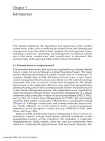
electricity, as shown in Figure 1.3. These rivers are also the migration
route for hatchery and wild salmon, so there is a clear potential for
conflict between different uses of the rivers. The dams were
constructed with bypass systems for the salmon, but there has been
concern nevertheless about salmon mortality rates in passing
downstream, with some studies suggesting losses as high as 85% of
hatchery fish in just portions of the river.
Figure 1.3 Map of the Columbia River Basin showing the location of dams.
Primary releases of pit-tagged salmon were made in 1993 and 1994 above
Lower Granite Dam, with recoveries at Lower Granite Dam and Little Goose
Dam in 1993, and at these dams plus Lower Monumental Dam in 1994.
In order to get a better understanding of the causes of salmon
mortality, a major study was started in 1993 by the National Marine
Fisheries Service and the University of Washington to investigate the
use of modern mark-recapture methods for estimating survival rates
through both the entire river system and the component dams. The
methodology was based on theory developed by Burnham et al.
(1987) specifically for mark-recapture experiments for estimating the
survival of fish through dams, but with modifications designed for the
application in question (Dauble et al., 1993). Fish are fitted with
Passive Integrated Transponder (PIT) tags which can be uniquely
identified at downstream detection stations in the bypass systems of
dams. Batches of tagged fish are released and their recoveries at
© 2001 by Chapman & Hall/CRC
detection stations are recorded. Using special probability models, it

is then possible to use the recovery information to estimate the
probability of a fish surviving through different stretches of the rivers
and the probability of fish being detected as they pass through a dam.
In 1993 a pilot programme of releases were made to (a) field test
the mark-recapture method for estimating survival, including testing
the assumptions of the probability model; (b) identify operational and
logistic constraints limiting the collection of data; and (c) determine
whether survival estimates could be obtained with adequate precision.
Seven primary batches of 830 to 1442 hatchery yearling chinook
salmon (Oncorhynchus tshawytscha) were released above the Lower
Granite Dam, with some secondary releases at Lower Granite Dam
and Little Goose Dam to measure the mortality associated with
particular aspects of the dam system. It was concluded that the
methods used will provide accurate estimates of survival probabilities
through the various sections of the Columbia and Snake Rivers
(Iwamoto et al., 1994).
The study continued in 1994 with ten primary releases of hatchery
yearling chinook salmon (O. tshawytscha) in batches of 542 to 1196,
one release of 512 wild yearling chinook salmon, and nine releases of
hatchery steelhead salmon (O. mykiss) in batches of 1001 to 4009, all
above the first dam. The releases took place over a greater
proportion of the juvenile migration period than in 1993, and survival
probabilities were estimated for a larger stretch of the river. In
addition, 58 secondary releases in batches of 700 to 4643 were made
to estimate the mortality associated with particular aspects of the dam
system. In total, the records for nearly 100,000 fish were analysed so
that this must be one of the largest mark-recapture study ever carried
out in one year with uniquely tagged individuals. From the results
obtained the researchers concluded that the assumptions of the
models used were generally satisfied and reiterated their belief that

these models permit the accurate estimation of survival probabilities
through individual river sections, reservoirs and dams on the Snake
and Columbia Rivers (Muir et al., 1995).
In terms of the three types of study that were defined in Section
1.1, the mark-recapture experiments on the Snake River in 1993 and
1994 can be thought of as part of a baseline study because the main
objective was to assess this approach for estimating survival rates of
salmon with the present dam structures with a view to assessing the
value of possible modifications in the future. Estimating survival rates
for populations living outside captivity is usually a difficult task, and
this is certainly the case for salmon in the Snake and Columbia
Rivers. However, the estimates obtained by mark-recapture seem
quite accurate, as is indicated by the results shown in Table 1.2.
© 2001 by Chapman & Hall/CRC
Table 1.2 Estimates of survival probabilities for ten
releases of hatchery yearling chinook salmon made
above the Lower Granite Dam in 1994 (Muir et al.,
1995). The survival is through the Lower Granite Dam,
Little Goose Dam and Lower Monumental Dam. The
standard errors shown with individual estimates are
calculated from the mark-recapture model. The
standard error of the mean is the standard deviation of
the ten estimates divided by %10
Release Number Survival Standard
Date Released Estimate Error
16-Apr 1189 0.688 0.027
17-Apr 1196 0.666 0.028
18-Apr 1194 0.634 0.027
21-Apr 1190 0.690 0.040
23-Apr 776 0.606 0.047

26-Apr 1032 0.630 0.048
29-Apr 643 0.623 0.069
1-May 1069 0.676 0.056
4-May 542 0.665 0.094
10-May 1048 0.721 0.101
Mean 0.660 0.011
Future objectives of the research programme include getting a
good estimate of the survival rate of salmon for a whole migration
season for different parts of the river system, allowing for the
possibility of time changes and trends. These objectives pose
interesting design problems, with the need to combine mark-recapture
models with more traditional finite sampling theory, as discussed in
Chapter 2.
This example is unusual because of the use of the special mark-
recapture methods. It is included here to illustrate the wide variety of
statistical methods that are applicable for solving environmental
problems
in this case improving the survival of salmon in a river that
is used for electricity generation.
Example 1.4 A Large-Scale Perturbation Experiment
Predicting the responses of whole ecosystems to perturbations is one
of the greatest challenges to ecologists because this often requires
experimental manipulations to be made on a very large-scale. In
many cases small-scale laboratory or field experiments will simply not
necessarily demonstrate the responses obtained in the real world. For
© 2001 by Chapman & Hall/CRC
this reason a number of experiments have been conducted on lakes,
catchments, streams, and open terrestrial and marine environments.
Although these experiments involve little or no replication, they do
indicate the response potential of ecosystems to powerful

manipulations which can be expected to produce massive unequivocal
changes (Carpenter et al., 1995). They are targeted studies as
defined in Section 1.1.
Carpenter et al. (1989) discussed some examples of large-scale
experiments involving lakes in the Northern Highlands Lake District of
Wisconsin in the United States. One such experiment, which was part
of the Cascading Trophic Interaction Project, involved removing 90%
of the piscivore biomass from Peter Lake and adding 90% of the
planktivore biomass from another lake. Changes in Peter Lake over
the following two years were then compared with changes in Paul
Lake, which is in the same area but received no manipulation.
Studies of this type are often referred to as having a before-after-
control-impact (BACI) design, of a type that is discussed in Chapter 6.
One of the variables measured at Peter Lake and Paul Lake was
the chlorophyll concentration in mg/m
3
. This was measured for ten
samples taken in June to August 1984, for 17 samples taken in June
to August 1985, and for 15 samples taken in June to August 1986.
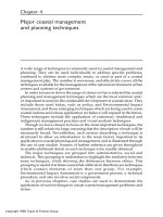
The manipulation of Peter Lake was carried out in May 1985. Figure
1.4 shows the results obtained. In situations like this the hope is that
time effects other than those due to the manipulation are removed by
taking the difference between measurements for the two lakes. If this
is correct, then a comparison between the mean difference between
the lakes before the manipulation with the mean difference after the
manipulation gives a test for an effect of the manipulation.
Before the manipulation, the sample size is 10 and the mean
difference (treated - control) is -2.020. After the manipulation the
sample size is 32 and the mean difference is -0.953. To assess
whether the change in the mean difference is significant, Carpenter et

al. (1989) used a randomization test. This involved comparing the
observed change with the distribution obtained for this statistic by
randomly reordering the time series of differences, as discussed
further in Section 4.6. The outcome of this test was significant at the
5% level so they concluded that there was evidence of a change.
© 2001 by Chapman & Hall/CRC
Figure 1.4 The outcome of an intervention experiment in terms of
chlorophyll concentrations (mg/m
3
). Samples 1 to 10 were taken in June to
August 1984, samples 11 to 27 were taken from June to August 1985, and
samples 28 to 42 were taken in June to August 1986. The treated lake
received a food web manipulation in May 1985, between samples number
10 and 11 (as indicated by a broken vertical line).
A number of other statistical tests to compare the mean differences
before and after the change could have been used just as well as the
randomization test. However, most of these tests may be upset to
some extent by correlation between the successive observations in
the time series of differences between the manipulated and the control
lake. Because this correlation will generally be positive it has the
tendency to give more significant results than should otherwise occur.
From the results of a simulation study, Carpenter et al. (1989)
suggested that this can be allowed for by regarding effects that are
significant between the 1 and 5% level as equivocal if correlation
seems to be present. From this point of view the effect of the
manipulation of Peter Lake on the chlorophyll concentration is not
clearly established by the randomization test.
This example demonstrates the usual problems with BACI studies.
In particular:
(a) the assumption that the distribution of the difference between Peter

Lake and Paul Lake would not have changed with time in the
© 2001 by Chapman & Hall/CRC
absence of any manipulation is not testable, and making this
assumption amounts to an act of faith; and
(b) the correlation between observations taken with little time between
them is likely to be only partially removed by taking the difference
between the results for the manipulated lake and the control lake,
with the result that the randomization test (or any simple alternative
test) for a manipulation effect is not completely valid.
There is nothing that can be done about problem (a) because of
the nature of the situation. More complex time series modelling offers
the possibility of overcoming problem (b), but there are severe
difficulties with using these techniques with the relatively small sets of
data that are often available. These matters are considered further in
Chapters 6 and 8.
Example 1.5 Ring Widths of Andean Alders
Tree ring width measurements are useful indicators of the effects of
pollution, climate, and other environmental variables (Fritts, 1976;
Norton and Ogden, 1987). There is therefore interest in monitoring
the widths at particular sites to see whether changes are taking place
in the distribution of widths. In particular, trends in the distribution may
be a sensitive indicator of environmental changes.
With this in mind, Dr Alfredo Grau collected data on ring widths for
27 Andean alders (Alnus acuminanta) on the Taficillo Ridge at an
altitude of about 1700 m in Tucuman, Argentina, every year from 1970
to 1989. The measurements that he obtained are shown in Figure
1.5. It is apparent here that over the period of the study the mean
width decreased, as did the amount of variation between individual
trees. Possible reasons for a change of the type observed here are
climate changes and pollution. The point is that regularly monitored

environmental indicators such as tree ring widths can be used to
signal changes in conditions. The causes of these changes can then
be investigated in targeted studies.
© 2001 by Chapman & Hall/CRC