RELATIONAL MANAGEMENT and DISPLAY of SITE ENVIRONMENTAL DATA - PART 5 ppsx
Bạn đang xem bản rút gọn của tài liệu. Xem và tải ngay bản đầy đủ của tài liệu tại đây (2.56 MB, 82 trang )
PART FIVE - USING THE DATA
© 2002 by CRC Press LLC
CHAPTER 18
DATA SELECTION
An important key to successful use of an EDMS is to allow users to easily find the data they
need. There are two ways for the software to assist the user with data selection: text-based and
graphical. With text-based queries, the user describes the data to be retrieved using words,
generally in the query language of the software. Graphical queries involve selecting data from a
graphical display such as a graph or a map. Query-by-form is a hybrid technique that uses a
graphical interface to make text-based selections.
TEXT-BASED QUERIES
There are two types of text-based queries: canned and ad hoc. The trade-off is ease of use vs.
flexibility.
Canned queries
Canned queries are procedures where the query is prepared ahead of time, and the retrieval is
done the same way each time. An example would be a specific report for management or
regulators, which is routinely generated from a menu selection screen. The advantage of canned
selections is that they can be made very easy to use since they involve a minimum of choices for
the user. The goal of this process is to make it easy to quickly generate the output that will be
required most of the time by most of the users. The EDMS should make it easy to add new canned
queries, and to connect to external data selection tools if required. Figure 85 shows an example of
a screen from Access from which users can select pre-made queries. The different icons next to the
queries represent the different query types, including select, insert, update, and delete. The user can
execute a query by double-clicking on it. Queries that modify data (action queries), such as insert,
update, and delete, display a warning dialog box before performing the action. Other than with the
icons, this screen does not separate selection queries from action queries, which results in some
risk in the hands of inexperienced or careless users.
© 2002 by CRC Press LLC
Figure 85 - Access database window showing the Queries tab
Ad hoc queries
Sometimes it is necessary to generate output with a format or data content that was not
anticipated in the system design. Text selections of this type are called ad hoc queries (“ad hoc” is
a Latin term meaning “for this”). These are queries that are created when they are needed for a
particular use. This type of selection is more difficult to provide the user, especially the casual
user, in a way that they can comfortably use. It usually requires that users have a good
understanding of the structure and content of the database, as well as a medium to high level of
expertise in using the software, in order to perform ad hoc text-based queries. The data model
should be included with the system documentation to assist them in doing this.
Unfortunately, ad hoc queries also expose a high level of risk that the data retrieved may not
be valid. For example, the user may not include the units for analyses, and the database may
contain different units for a single parameter sampled at different times. The data retrieved will be
invalid if the units are assumed to be the same, and there is no visible indication of the problem.
This is particularly dangerous when the user is not seeing the result of the query directly, but using
the data indirectly to generate some other result such as statistics or a contour map. In general, it is
desirable to formalize and add to the menu as wide a variety of correctly formatted retrievals as
possible. Then casual users are likely to get valid results, and “power users” can use the ad hoc
queries only as necessary.
Figure 86 shows an example of creation of an ad hoc text-based query. The user has created a
new query, selected the tables for display, dragged the fields from the tables to the grid, and
entered selection criteria. In this case, the user has asked for all “Sulfate” results for the site “Rad
Industries” where the value is > 1000. Access has translated this into SQL, which is shown in the
second panel, and the user can toggle between the two. The third panel shows the query in
datasheet view, which displays the selected data. The design and SQL views contain the same
information, although in Access it is possible to write a query, such as a union query, that can’t be
displayed in design view and must be shown in SQL. Some advanced users prefer to type in the
SQL rather than use design view, but even for them the drag and drop can save typing and
minimize errors.
© 2002 by CRC Press LLC
Figure 86 - A text-based query in design, SQL, and datasheet views
GRAPHICAL SELECTION
A second selection type is graphical selection. In this case, the user generates a graphical
display, such as a map, of a given site, selects the stations (monitoring wells, borings, etc.), then
retrieves associated analytical data from the database.
© 2002 by CRC Press LLC
Figure 87 - Interactive graphical data selection
Figure 88 - Editing a well selected graphically
© 2002 by CRC Press LLC
Figure 89 - Batch-mode graphical data selection
Geographic Information System (GIS) programs such as ArcView, MapInfo, and Enviro Spase
provide various types of graphical selection capability. Some map add-ins that can be integrated
with database management and other programs, such as MapObjects and GeoObjects, also offer
this feature.
There are two ways of graphically selecting data, interactive and batch. In Figure 87 the user
has opened a map window and a list window showing a site and some monitoring wells. The user
then double-clicked on one of the wells on the map, and the list window scrolled to show some
additional information on the well.
In Figure 88 a well was selected graphically, then the user called up an editing screen to view
and possibly change data for that well. The capability of working with data in its spatial context
can be a valuable addition to an EDMS.
In Figure 89 the user wanted to work with wells in or near two ponds. The user dragged a
rectangle to select a group of wells, and then individually selected another. Then the user asked the
software to create a list of information about those wells, which is shown on the bottom part of the
screen. In this case the spatial component was a critical part of the selection process.
Selection based on distance from a point can also be valuable. The point can be a specific
object, such as a well, or any other location on the ground, such as a proposed construction
location. The GIS can help you perform these selections.
Other types of graphical selection include selection from graphs and selections from cross
sections. Some graphics and statistics programs allow you to create a graph, and then click on a
point on the graph and bring up information about that point, which may represent a station,
sample, or analysis. GIS programs that support cross section displays can provide a similar feature
where a user can click on a soil boring in a cross section, and then call up data from that boring, or
a specific sample for that boring.
© 2002 by CRC Press LLC
Figure 90 - Example of query-by-form
QUERY-BY-FORM
A technique that works well for systems with a variety of different user skill levels is query-
by-form, or QBF. In this technique, a form is presented to the user with fields for some of the data
elements that are most likely to be used for selection. The user can fill out as many of the fields as
needed to select the subset that the user is interested in. The software then creates a query based on
the selection criteria. This query can then be used as the basis for a variety of different lists,
reports, graphs, maps, or file exports. Figure 90 shows an example of this method.
© 2002 by CRC Press LLC
Figure 91 - Query-by-form screen showing selection criteria for different data levels
In this example, the user has selected Analyses in the upper right corner. Along the left side
the user selected “Rad Industries” as the site, and “MW-1” as the station name. In the center of the
screen, the user has selected a sample date range of greater than 1/1/1985, and “Sulfate” as the
parameter. The lower left of the screen indicates that there are 16 records that match these criteria,
meaning that there are 16 sulfate measurements for this well for this time period. When the user
selected List, the form at the bottom of the screen was displayed showing the results.
To be effective, the form for querying should represent the data model, but in a way that feels
comfortable to the user. Also, the screen should allow the user to see the selection options
available. Figure 91 shows four different versions of a screen allowing users to make selections at
four different levels of the data hierarchy.
The more defined the data model, the easier it is to provide advanced user-friendly selection.
The Access query editor is very flexible, and will work with any tables and fields that might be in
the database. However, the user has to know the values to enter into the selection criteria. If the
fields are well defined and won’t change, then a screen like that shown in Figures 90 and 91 can
provide selection lists to select values from. Figure 92 shows an example of a screen showing the
user a list of parameter names to choose from.
© 2002 by CRC Press LLC
Figure 92 - Query-by-form screen showing data choices
One final point to be emphasized is the reliance of data quality on good selection practices.
This was discussed above and in Chapter 15. Improper selection and display can result in data that
is easy to misinterpret. Great care must be taken in system design, implementation, and user
training so that the data retrieved accurately represents the answer to the question the user intended
to ask.
© 2002 by CRC Press LLC
CHAPTER 19
REPORTING AND DISPLAY
It takes a lot of work to build a good database. Because of this, it makes sense to get as much
benefit from the data as possible. This means providing data in formats that are useful to as many
aspects of the project as possible, and printed reports and other displays are one of the primary
output goals of most data management projects. This chapter covers a variety of issues for reports
and other displays. Graph displays are described in Chapter 20. Cross sections are discussed in
Chapter 21, and maps and GIS displays in Chapter 22. Chapter 23 covers statistical analysis and
display, and using the EDMS as a data source for other programs is described in Chapter 24.
TEXT OUTPUT
Whether the user has performed a canned or ad hoc query, the desired result might be a tabular
display. This display can be viewed on the screen, printed, saved to a file, or copied to the
clipboard for use in other applications. Figure 93 is an example of this type of display. This is the
most basic type of retrieval. This is considered unformatted output, meaning that the data is there,
but there is no particular presentation associated with it.
Figure 93 - Tabular display of output from the selection screen
© 2002 by CRC Press LLC
Figure 94 - Banded report for printing
FORMATTED REPORTS
Once a selection has been made, another option is formatted output. The data can be sent to a
formatted report for printing or electronic distribution. A formatted report is a template designed
for a specific purpose and saved in the program. The report is based on a query or table that
provides the data, and the report form provides the formatting.
Standard (banded) reports
Figure 94 is an example of a report formatted for printing. This example shows a standard
banded report, where the data at different parent-child levels is displayed in horizontal bands
across the page. This is the easiest type of report to create in many database systems, and is most
useful when there is a large amount of information to present for each data element, because one or
more lines can be dedicated to each result.
Cross-tab reports
The next figure, Figure 95, shows a different organization called a cross-tab or pivot table
report. In this layout, one element of the data is used to create the headers for columns. In this
example, the sample event information is used as column headers.
© 2002 by CRC Press LLC
Figure 95 - Cross-tab report with samples across and parameters down
Figure 96 - Cross-tab report with parameters across and samples down
Figure 96 is a cross-tab pivoted the other way, with parameters across and sample events
down. In general, cross-tab reports are more compact than banded reports because multiple results
can be shown on one line.
© 2002 by CRC Press LLC
Figure 97 - Data display options
Cross-tab reports provide a challenge regarding the display of field data when multiple field
observations must be displayed with the analytical data. Typically there will be one result for each
analyte (ignoring dilutions and reanalyses), but several observations of pH for each sample. In a
cross-tab, the additional pH values can be displayed either as additional columns or additional
rows. Adding rows usually takes less space than additional columns, so this may be preferred, but
either way the software needs to address this issue.
FORMATTING THE RESULT
There are a number of options that can affect how the user sees the data. Figure 97 shows a
panel with some of these options for how the data might be displayed.
The user can select which regulatory limit or regulatory limit group to use for comparison,
how to handle non-detected values, how to display graphs and handle field data, whether to include
calculated parameters, how to display the values and flags, how to format the date and time, and
whether to convert to consistent units and display regulatory limits.
Regulatory limit comparison
For investigation and remediation projects, an important issue is comparison of analytical
results to regulatory limits or target levels. These limits might be based on national regulations
such as federal drinking water standards, state or local government regulations, or site-specific
goals based on an operating permit or Record of Decision (ROD). Project requirements might be to
display all data with exceedences highlighted, or to create a report with only the exceedences. For
most constituents, the comparison is against a maximum value. For others, such as pH, both an
upper and a lower limit must be met.
The first step in using regulatory limits is to define the limit types that will be used. Figure 98
shows a software screen for doing this. The user enters the regulatory limit types to be used, along
with a code for each type.
The next step is to enter the limits themselves. Figure 99 shows a form for doing this. Limits
can be entered as either site-specific or for all sites. For each limit, the matrix, parameter, and limit
type are entered, along with the upper and lower limits and units. The regulatory limit units are
particularly important, and must be considered in later comparison, and should be taken into
consideration in conversion to consistent units as described below.
There is one complication that must be addressed for limit comparison to be useful for many
project requirements. Often the requirement is for different parameters, or groups of parameters, to
be compared to different limit types on the same report. For example, the major ions might be
compared to federal drinking water standards, but the organics may be compared to more stringent
local or site-specific criteria. This requires that the software provide a feature to allow the use of
different limits for different parameters. Figure 100 shows a screen for doing this. The user enters a
name for the group, and then selects limits from the various limit types to use in that group.
© 2002 by CRC Press LLC
Figure 98 - Form for defining regulatory limit types
Figure 99 - Form for entering regulatory limits
Figure 100 - Form for defining regulatory limit groups
© 2002 by CRC Press LLC
Figure 101 - Selection of regulatory limit or group for reporting
After the limits and groups have been defined, they can be used in reporting. Figure 101 shows
a panel from the selection screen where the user is selecting the limit type or group for comparison.
The list contains both the regulatory limit types and the regulatory limit groups, so either one can
be used at report time. The software code should be set up to determine which type of limit has
been selected, and then retrieve the proper data for comparison.
Value and flag
Analytical results contain much more information than just the measured value. A laboratory
deliverable file may contain 30 or more fields of data for each analysis. In a banded report there is
room to display all of this data. When the result is displayed in a cross-tab report, there is only one
field for each result, but it is still useful to display some of this additional information. The items
most commonly involved in this are the value, the analytical flag, and the detection limit. Different
EDMS programs handle this in different ways, but one way to do it is using fields for reporting
factor and reporting basis that are based on the analytical flag. Another way to do it is to have a
text field for each analysis containing exactly the formatting desired. Examples of reporting factor
and reporting basis values, and how each result might look, are shown in the following table:
Basis
code
Reporting basis Reporting
factor
Value Flag Detection
limit
Result
v Value only 1 3.7 v 0.1 3.7
f Flag only 1 3.7 v 0.1 v
b Both value and flag 1 3.7 v 0.1 3.7 v
l Less than sign (<) and
detection limit or value
1 3.7 u 0.1 < 0.1
g Greater than sign (>) and
detection limit or value
1 3.7 u 0.1 > 0.1
d Detection limit (times factor)
and flag
1 3.7 u 0.1 0.1 u
d Detection limit (times factor)
and flag
.5 3.7 u 0.1 0.05 u
a Average of values 1 3.7 v 0.1 1.9
m Dash (-) only 1 3.7 v 0.1 -
The next table shows examples of some analytical flags and how the reporting factor and
reporting basis might be assigned to each.
© 2002 by CRC Press LLC
Flag code Flag Reporting factor Reporting basis
b Analyte detected in blank and sample 1 v
c Coelute 1 v
d Diluted 1 v
e Exceeds calibration range 1 v
f Calculated from higher dilution 1 v
g Concentration > value reported 1 g
h Result reported elsewhere 1 f
i Insufficient sample 0 v
j Est. value; conc. < quan. limit 1 b
l Less than detection limit 1 l
m Matrix interference 1 v
n Not measured 0 v
q Uncertain value 1 v
r Unusable data 0 f
s Surrogate 1 v
t Trace amount 1 d
u Not detected 0.5 l
v Detected value 1 v
w Between CRDL/IDL 1 v
x Determined by associated method 1 v
y Calculated value 0 v
z Unknown 1 v
Finally, analyses can often have multiple flags, for example “uj,” but the result can only be
displayed one way. The software needs to have an established priority for the reporting basis so
that the display is based on the highest priority format. Based on the previous basis code values, an
example of the priority might be: f, l, g, b, d, v, a, and m. This means that for a flag of “bj” the
basis codes would be “v” (from the “b” flag) and “b” (from the “j” flag). The “b” basis would have
preference, so a less than sign (<) and the value would be displayed.
Non-detects
When laboratories analyze for a constituent, it may or may not be found. If it is not found, it is
referred to as not detected, or a non-detect. The various different detection limits used by
laboratories are discussed in Chapter 12. If the result is not detected at the appropriate limit, the lab
should flag (qualify) the data with a flag such as “u” for “undetected.” It should also report the
detection limit and the limit type. It may or may not place the detection limit in the value field.
In reporting and otherwise working with non-detects, they can be handled in several ways. In a
full, banded report, the value, flag, detection limit, and detection limit type can all be reported. In a
cross-tab report, or an export such as an XYZ file for contouring, there is no room for that. There
are several ways to handle non-detects. Often a combination of these is used.
Ignore them – Analyses for which the constituent was not detected can be excluded. This is
generally not a good idea, since the fact that the constituent wasn’t detected is useful information.
Display the value – The software can display the value provided by the laboratory, but this is
risky, because the laboratory may or may not place the detection limit in the value field. It has the
advantage of being easy to implement, because the report can be based on only one field.
© 2002 by CRC Press LLC
Figure 102 - Form for defining calculated parameters
Display the detection limit – It makes sense to display the detection limit for non-detected
values and the value if there was a detection. This is more complicated to program than just basing
the report on the value field, because the software has to look at the analysis record and determine
which field to display, either using an IF statement (or more likely the slightly different immediate
IIF) or using program code.
Display the limit and qualify it – If the limit is displayed, it is helpful to qualify it in the
report, either by displaying a less than sign (<) or the flag. To do this only for the non-detects
requires special handling in the software.
Apply a factor to the limit – Sometimes a numerical factor is applied to the detection limit
before it is displayed. A common factor is one half, although others are sometimes used. The
thinking is that the true value is somewhere between the detection limit and zero, so one half is a
good guess. This can be useful for estimating volumes of a material, or for other statistical
calculations.
Display a zero – A variation on using a factor is to use a zero for non-detects. This is usually
not correct technically, but can be useful in some applications like contour mapping. If you do use
a zero value in contouring, be sure to do so with care. The value is not really a zero, but is less than
a specific value (the detection limit), and setting it to zero could be misleading, especially if the
detection limit is highly elevated, and the real value could be different enough from zero to affect
the surface. Another option for contouring is to set the value to the indeterminate value, which is
the value (such as -99999) that the contouring program ignores in calculating the surface, but then
you are throwing away the useful information that the value is low. Some, but not many,
contouring programs allow you to specify that the value is less than a certain amount, and then the
software constrains the surface based on that information. That is the best solution if it is available.
Which approach is best for displaying non-detects depends on the use of the data. It is
important that data users be aware of how the result is being displayed.
Calculated fields
Sometimes it is helpful to display data that is based on calculations using data that is in the
database. These are referred to as calculated fields or derived values. These are results that are not
contained in the database, but are generated “on the fly” at retrieval time. The software can provide
a system for defining and calculating these results. Figure 102 shows an example of how this might
be presented.
© 2002 by CRC Press LLC
In this screen, the user has specified that the software is to calculate the mass of the total
dissolved solids for a sample. The input parameters have been selected as the total dissolved solids
concentration times the effluent volume. The result must then be scaled to the output units of
kilograms by dividing by one million. The screen is also asking for a nesting order, which
determines the order in which multiple calculations are to be performed, allowing complicated
multi-step calculations with many parameters if necessary. There is also a checkbox to enable and
disable the calculated field, so that a particular calculation can be turned off and on without
deleting it.
Consistent units
It is possible that different results for the same parameter in the database might be in different
units. This can be avoided at import time, as described in Chapter 13, but that is not always
desirable. When the data is displayed in a banded report with one or more lines per result, and the
units displayed, then multiple units may not be a problem, since a unit is shown with each value. In
a cross-tab report, or if only the numbers (and not the units) are being retrieved for use in statistics,
graphing, or mapping, then it is mandatory to convert to consistent units. A good approach is to
define in the software the target units for each parameter and matrix. Matrix is important because
the units for different matrices usually should be different. For example, in water the concentration
of a constituent like a metal is reported as mass per unit volume, such as milligrams per liter, while
for a solid such as soil, it is in mass per mass, such as milligrams per kilogram or parts per million.
A screen for defining target units for each parameter is shown in Figure 103.
The next step is to define all of the conversion factors necessary to do the conversions. This is
also shown in Figure 103. Conversion of different units of the same scale, such as from milligrams
per liter to micrograms per liter, is pretty straightforward. Not all conversions are this simple,
however, and great care must be taken in converting between different types of measure. For
example, the laboratory may express measurements of radioactive materials like radium
226
in
activity, such as picocuries per gram. In order to determine how much material is there, it is useful
to have the data in mass units, such as milligrams per kilogram. This conversion, however, depends
on a number of factors, such as the isotopic mix, physical properties of the sample, and so on, and
consequently is at best site-specific, and at worst involves complicated statistical calculations. Be
sure you know what you are doing before you go too far with unit conversions.
Once the desired concentration and conversion factors have been defined, the software can
perform the conversion. It is obvious that the value should be converted, but usually you will also
want to convert other related information, such as the detection limit, regulatory limits used for
comparison, and so on.
Other issues
There are a number of other issues that arise in formatting the data to satisfy project needs.
These include handling of decimal places and date and time formatting.
Handling of decimal places, or significant figures, is an issue that is not done well in many
software programs. Try this experiment. Open a new database in Excel. In one of the cells, type in
3.00, and press Enter. The zeros go away. Access and other programs lose trailing zeros the same
way. This results in lost information. If the analysis was to two decimal places, then those zeros
should be displayed. There are two ways to handle this in an Access-based database. One is to
store the value as a text string, rather than as a number. The other is to store the number of decimal
places in a separate field, and combine the two if necessary at retrieval time using a user-defined
function.
© 2002 by CRC Press LLC
Figure 103 - Forms for defining units by parameter and matrix, and conversion between units
The issue of date and time formatting is related to the way that the data management software
stores dates and times, and how you want them displayed. For example, Access combines dates and
times into one field. This field is a numeric field, with the whole number (left of the decimal point)
representing the date. Internally this is stored as the number of days since Dec. 31, 1899, so a value
of 1 is Jan. 1, 1900, and Jan. 1, 2002 is 37257. The decimal portion of the date number (right of
the decimal point) represents the time, starting at midnight. For example, a value of .5 is 12:00 PM
(noon) and 8:30 AM is .3541666667. This combination of date and time storage is different from
some other systems, such as dBase and FoxPro, where the date and time are stored in separate
fields. For environmental projects, the date is nearly always important, but the time may or may not
be. For example, for soil samples taken once, the time during the day that they were taken may not
be important, but for air samples taken every hour, it certainly would be. For systems like Access
that combine the date and time, it is useful to have a feature to turn the display of the time on and
off as appropriate for the data being displayed. Reports can be formatted to display the date and
time field in different fields if desired.
© 2002 by CRC Press LLC
Sample Point ->
Matrix: Water Sample Date ->
MW-1
2/26/1981
MW-1
4/20/1981
Parameters Reg. Limit Units
Field pH s.u. 7.8 7.9
Iron (Ferrous) mg/l 0.35 0.10 bj
Nitrate mg/l 1.7 < 1.0
Potassium mg/l 6.9 6.6
Sulfate DW 400 mg/l
1255
1400
Reg. Limits: DW - Federal drinking water standards
Sample Point ->
Matrix: Water Sample Date ->
MW-1
2/26/1981
MW-1
4/20/1981
Parameters Units
Field pH s.u. 7.8 7.9
Iron (Ferrous) mg/l 0.35 0.1
Nitrate mg/l 1.7 1
Potassium mg/l 6.9 6.6
Sulfate mg/l 1255 1400
Figure 104 - Reports with different levels of formatting for performance comparison
Formatting and performance
Keep in mind that asking the software to perform sophisticated formatting comes at a cost. In
Figure 104, the panel on the top has formatted values and comparison to regulatory limits. Notice
that a regulatory limit is displayed for sulfate, and both sulfate values are bolded and underlined
because they exceed this limit. Also, for 4/20/1981 the value for iron shows the value and
analytical flags, and the value for nitrate shows “<” and the detection limit. This retrieval for 315
records takes 17 seconds. The panel on the bottom displays only the numbers, with no comparison
to limits, and takes 1.5 seconds. In data management (as in most everything else) nothing is free.
INTERACTIVE OUTPUT
In the past, nearly all of the focus of data management has been on generating printed reports.
As data management software evolves, it is now becoming possible to work interactively with the
data in ways that before were either not possible or not time-effective.
Figure 105 shows an example of this type of interactive display. The software is showing the
environmental data in a TreeView display. This display, which is similar to the Windows Explorer
display, shows sites at the highest level, then stations, samples, and analyses. At each level, the
most pertinent data is displayed. This type of display lets the user “drill down” to find a particular
result quickly, even in a large database.
© 2002 by CRC Press LLC
Figure 105 - TreeView display of site data
ELECTRONIC DISTRIBUTION OF DATA
Often the person managing the data is not the person using it. The best approach is for
everyone that needs the data to have direct access to it through the EDMS. For various reasons,
such as cost and location, this is not always possible. There are several ways to overcome this. One
is to make the data available more generally, such as through Web access. Another way is through
electronic distribution of reports. The Adobe Portable Document Format (PDF) and the free PDF
reader are a convenient way to distribute reports. Users create the report that they want in the
EDMS, and then print it to the PDF format using Acrobat for distribution. Recipients of the report
can use the free Acrobat reader to see it, formatted the way the database user intended.
© 2002 by CRC Press LLC
CHAPTER 20
GRAPHS
There’s an old saying that a picture is worth a thousand words. In many situations, presenting
data in a graphical display makes the information much more understandable. A well-designed
graph of the data in a table can be many times more informative than the table alone. This chapter
and the next two describe and show a variety of graphic displays that can be used to present
environmental data. This chapter discusses traditional graphs. Other graphic displays, such as maps
and cross sections, are discussed in the following two chapters.
GRAPH OVERVIEW
There’s a good and a bad side to graphs. They can be used to display data in a format
conducive to greater understanding. They can also be confusing, misleading, or even dishonest. An
excellent book by Tufte (1983) provides a wealth of information on various aspects of graphical
data display, including graphs and maps. According to Tufte, graphical displays should:
Show the data
Induce the viewer to think about the substance rather than about methodology, graphic
design, the technology of graphic production, or something else
Avoid distorting what the data has to say
Present many numbers in a small space
Make large data sets coherent
Encourage the eye to compare different pieces of data
Reveal the data at several levels of detail, from a broad overview to fine structure
Serve a reasonably clear purpose: description, exploration, tabulation, or decoration
Be closely integrated with the statistical and verbal description of a data set
In addition, Tufte provides the following six principles of graphical integrity:
The representation of numbers, as physically measured on the surface of the graphic itself,
should be directly proportional to the numerical quantities expressed.
Clear, detailed, and thorough labeling should be used to defeat graphical distortions and
ambiguity. Write out explanations of the data on the graphic itself. Label important events
in the data.
Show data variation, not design variation.
In time-series displays of money, deflated and standardized units of monetary
measurement are nearly always better than nominal units.
The number of information-carrying (variable) dimensions depicted should not exceed the
number of dimensions in the data.
Graphics must not quote data out of context.
© 2002 by CRC Press LLC
Following these two sets of guidelines will greatly increase your chance of creating good
graphical displays. Additional general information on graphs can be found in Milne (1992), and
information specific to environmental graphing in Sara (1994, pp. 11-19 to 11-28).
GENERAL CONCEPTS
Because graphing software is so accessible and easy to use, there is a tendency to throw
together a graph of a bunch of data and be done with it. If you try to follow Tufte’s guidelines
above, then clearly there is more to it than that, from making sure the data is amenable to the
graphing technique you will be using to confirming at the end that the graph communicates the
correct message. If you keep in mind the key concepts of creating a graph, rather than take them for
granted, your graphs will be much more effective.
Generally graphs present data with one data element graphed as a function of another.
Commonly the independent variable, which is often presented against the X (horizontal) axis, is
time, and the dependent variable, presented against the Y (vertical) axis, is the measured value. It
is also possible to plot one observed value against another. Sometimes the X-axis is called the
abscissa and the Y-axis is called the ordinate.
Data issues
Back in the day when graphs were created by hand, the person creating the graph was forced
to look at each data point, because he or she scaled it off and drew it on the graph. With automated
programs like Microsoft Excel and Golden Software’s Grapher, it is easy to create a graph without
giving it much thought. This can result in a graph that looks great, but, in the worst case, is totally
meaningless. For example, if you take a data set like the one graphed in Figure 106, and set the
scale to logarithmic as discussed below, Grapher will complain if some of the data has a zero value
and can’t be graphed, but Excel won’t. Those values may be important, and won’t be displayed in
either case, but with Excel you might not even know they are gone.
There are a number of other data issues that can trip you up in creating graphs. Chapter 19
discussed the importance of checking units during data retrieval. Use of non-detects and flagged
data must be done carefully. Duplicate data can also be a problem.
A good policy is to take a hard look at the data after it has been retrieved from the EDMS, but
before it is graphed. Look at every number, or if there is too much data to do that, sort in various
ways to understand the data ranges, relationships between different values, and so on. Time spent
doing this will be rewarded by better graphs, ones that you are more likely to be able to trust.
Coordinate systems
Graphing involves taking values and plotting them relative to some coordinate system. For
most graphs this is a Cartesian XY system, but other systems, such as polar and radial plots, are
possible. Think about which system will work best with your data and the message you are trying
to get across, rather than just using the default provided by the software.
Graph scales
The scales of the graph determine the spacing of the points relative to each axis. In the simple
case of an X-Y graph of two constituents against each other, the value range for each constituent
will be used as the scale for each axis. In the case of a time-sequence graph, one of the axes
(usually the horizontal one) is the time or date range, and the other is the value or values.
© 2002 by CRC Press LLC
0 200 400 600 800 1000 1200
U Tot
0
200
400
600
800
1000
1200
Ra 226
Parameter Comparison
0.1 1 10 100 1000
U Tot
0.1
1
10
100
1000
Ra 226
Parameter Comparison
Figure 106 - Comparison of linear vs. logarithmic scales
For the case where the data has a large dynamic range, or where the data is lognormally
distributed, a logarithmic scale on one or both axes may be appropriate. A graph with a
logarithmic scale on one axis and a linear scale on the other is called a semi-log plot, and one with
both axes logarithmic is called a log-log plot. The graph on the right side of Figure 106 shows a
log-log plot. The goal is to see the relationship between the two constituents in each sample. The
left graph shows the data graphed on a linear scale. Most of the data is clustered in the lower left,
and it is difficult to say what the relationship is. The right graph shows a logarithmic scale for both
constituents, and it is possible to see that there is a rough correlation between the two, and a sample
with a high value in one is likely to have a high value in the other. In fact, it appears that there may
be several populations with different linear relationships between the constituents, perhaps
representing different sources of the material. This was not at all apparent from the linear graph.
Labels and annotations
There are two basic types of labels and annotations, those associated directly with graph
elements, and those not. Examples of the first type are the scale labels and scale titles. Scale labels
identify positions along a scale axis. Usually there will be one set of labels per axis, such as the
numbers annotating the tic marks and the text label for the axis. Labels not associated with graph
elements include the graph title, legends, comments, and so on.
TYPES OF GRAPHS
Because graphics are so useful, people have developed many different types of graphs to best
represent their data. This section describes some of the most popular types of graphs, and the
following one shows some examples.
Line graphs – Line graphs are often used to represent data in a series. A grid is drawn, and
then one or more series of data are drawn on the grid. Lines are used to connect the points to
highlight trends and patterns. Often the horizontal axis (abscissa) is time, and the vertical axis
Whenever presenting a forecast, give a number and a date, but never both.
Rich (1996)
© 2002 by CRC Press LLC
(ordinate) is the value being compared, but this is not required. Line graphs are probably the most
common type of technical graph.
Bar graphs – Bar graphs, also called column graphs, are good for displaying increases and
decreases in quantity over a period of time. They work best when the amount of data to be
displayed is not large. As with line graphs, the horizontal axis is often time.
Area graphs – Area graphs are similar to line graphs, except the areas under the curve(s) are
filled.
Stacked graphs – A stacked graph is a variety of bar or (more commonly) area graph where
the values are stacked cumulatively rather than each starting at zero.
Scatter plots – A scatter plot is used for displaying two variables for each point against each
other. Scatter plots are very popular for technical data.
Box plots – Box plots are special bar graphs that show the minimum, maximum, mean, and
lower and upper quartiles for each data group.
Picture graphs – In picture graphs, the data is displayed with symbols rather than lines or
bars. These are sometimes used for business presentations, but are not commonly used for displays
of technical data.
Pie charts – A pie chart is a type of graph used to display the fractional parts of a whole like
slices of a pie, where the size, or more accurately the angular displacement, of each slice is based
on the percentage of the whole contributed by each value.
Surface plots – Surface plots are used to show one variable as a function of two others. They
are similar to contour displays used on maps, but the two independent variables can be something
other than map coordinates.
Rose diagram – A rose diagram is a circular graph of angular data. Angular measurements,
such as joint or cross-bed directions, are grouped by an angle range, such as 10° or 30°, and the
number of observations in each range are shown as distances from the center. Before designing a
rose diagram, you should examine the variability in the data and set the increments (angle range) to
be graphed appropriately. If the increment is too small for the data, then only “noise” is displayed.
If too coarse, the real variability is lost. An alternative way of drawing the rose diagram is to start
at the outer edge and increase the values toward the center. This often helps to define trends in
multi-modal data sets better than the more conventional approach (Mike Wiley, pers. comm.,
2002).
Polar plot – A polar plot is also a circular graph of angular data. Values as a function of angle
are shown as distances from the center, creating a line graph within a circle.
Maps – It’s important to remember that maps are a type of graph. Because maps have so many
special issues to discuss, they will be covered separately in Chapter 22. There are also many
opportunities for combining maps with traditional graphs to create visually rich and informative
displays.
GRAPH EXAMPLES
The following examples show graphs created by several different programs. Figure 107 shows
a number of graphs created with Microsoft Excel. Figure 108 shows some more technical graph
types created with Grapher from Golden Software.
The previous examples have used programs outside the EDMS. Figure 110 shows a fairly
typical graph of one parameter (sulfate) from two wells plotted as a function of time within an
EDMS program. Figure 111 shows a variation on the time sequence graph where data from several
years is folded onto one 12-month graph. This was done to help identify seasonality in the data.
© 2002 by CRC Press LLC