Species Sensitivity Distributions in Ecotoxicology - Section 2 pdf
Bạn đang xem bản rút gọn của tài liệu. Xem và tải ngay bản đầy đủ của tài liệu tại đây (1.93 MB, 158 trang )
© 2002 by CRC Press LLC
Section II
Scientific Principles and
Characteristics of SSDs
This section deals with theoretical and technical issues in the derivation of species
sensitivity distributions (SSDs). The issues include the assumptions underlying the
use of SSDs, the selection and treatment of data sets, methods of deriving distribu-
tions and estimating associated uncertainties, and the relationship of SSDs to dis-
tributions of exposure. A unifying statistical principle is presented, linking all current
definitions of risk that have been proposed in the framework of SSDs. Further,
methods for using SSDs for data-poor substances are proposed, based on effect
patterns related to the toxic mode of action of compounds. Finally, the issue of SSD
validation is addressed in this section. These issues are the basis for the use of SSDs
in setting environmental criteria and assessing ecological risks (Sections IIIA and B).
© 2002 by CRC Press LLC
Theory of Ecological Risk
Assessment Based on
Species Sensitivity
Distributions
Nico M. van Straalen
CONTENTS
4.1 Introduction
4.2 Derivation of Ecological Risk
4.3 Probability Generating Mechanisms
4.4 Species Sensitivity Distributions in Scenario Analysis
4.5 Conclusions
Acknowledgments
Abstract
— The risk assessment approach to environmental protection can be consid-
ered as a quantitative framework in which undesired consequences of potentially toxic
chemicals in the environment are identified and their occurrence is expressed as a relative
frequency, or a probability. Risk assessment using species sensitivity distributions
(SSDs) focuses on one possible undesired event, the exposure of an arbitrarily chosen
species to an environmental concentration greater than its no-effect level. There are two
directions in which the problem can be addressed: the forward approach considers the
concentration as given and aims to estimate the risk; the inverse approach considers the
risk as given and aims to estimate the concentration. If both the environmental concen-
tration (PEC) and the no-effect concentration (NEC) are distributed variables, the
expected value of risk can be obtained by integrating the product of the probability
density function of PEC and the cumulative distribution of NEC over all concentrations.
Analytical expressions for the expected value of risk soon become rather formidable,
but numerical integration is still possible. An application of the theory is provided,
focusing on the interaction between soil acidification and toxicity of metals in soil. The
analysis shows that the concentration of lead in soil that is at present considered a safe
reference value in the Dutch soil protection regulation may cause an unacceptably high
risk to soil invertebrate communities when soils are acidified from pH 6.0 to pH 3.5.
This is due to a strong nonlinear effect of lead on the expected value of risk with
decreasing pH. For cadmium the nonlinear component is less pronounced. The example
illustrates the power of quantitative risk assessment using SSDs in scenario analysis.
4
© 2002 by CRC Press LLC
4.1 INTRODUCTION
The idea of risk has proved to be an attractive concept for dealing with a variety of
environmental policy problems such as regulation of discharges, cleanup of contam-
inated land, and registration of new chemicals. The reason for its attractiveness seems
to be because of the basically quantitative nature of the concept and because it allows
a variety of problems associated with human activities to be expressed in a common
currency. This chapter addresses the scientific approach to ecological risk assess-
ment, with emphasis on an axiomatic and theoretically consistent framework.
The most straightforward definition of risk is
the probability of occurrence of
an undesired event
. As a probability, risk is always a number between 0 and 1,
sometimes multiplied by 100 to achieve a percentage. An actual risk will usually
lie closer to 0 than to 1, because undesired events by their nature are relatively rare.
For the moment, it is easiest to think of probabilities as relative frequencies, being
measured by the ratio of actual occurrences to the total number of occurrences
possible. The mechanisms generating probabilities will be discussed later in this
chapter.
In the scientific literature and in policy documents, many different definitions
of risk have been given. Usually, not only the occurrence of undesired events is
considered as part of the concept of risk, but also the magnitude of the effect. This
is often expressed as risk = (probability of adverse effect)
×
(magnitude of effect).
This is a misleading definition, because, as pointed out by Kaplan and Garrick
(1981), it equates a low probability/high damage event with a high probability/low
damage event, which are obviously two different types of events, not the same thing
at all. This is not to negate the importance of the magnitude of the effect; rather,
magnitude of effect should be considered
alongside
risk. This was pictured by
Kaplan and Garrick (1981) in their concept of the “risk curve”: a function that
defines the relative frequency (occurrence) of a series of events ordered by increasing
severity. So risk itself should be conceptually separated from the magnitude of the
effect; however, the
maximum acceptable risk
for each event will depend on its
severity.
When the above definition of risk is accepted, the problem of risk assessment
reduces to (1) specifying the undesired event and (2) establishing its relative inci-
dence. The undesired event that I consider the basis for the species sensitivity
framework is
a species chosen randomly out of a large assemblage is exposed to
an environmental concentration greater than its no-effect level
.
It must be emphasized that this endpoint is only one of several possible. Suter
(1993) has extensively discussed the various endpoints that are possible in ecological
risk assessments. Undesired events can be indicated on the level of ecosystems,
communities, populations, species, or individuals. Specification of undesired events
requires an answer to the question: what is it that we want to protect in the envi-
ronment? The species sensitivity distribution (SSD) approach is only one, narrowly
defined, segment of ecological risk assessment. Owing to its precise definition of
the problem, however, the distribution-based approach allows a theoretical and
quantitative treatment, which adds greatly to its practical usefulness.
© 2002 by CRC Press LLC
It is illustrative to break down the definition of our undesired event given the
above and to consider each part in detail:
•“
A species chosen randomly
” — This implies that species, not individuals,
are the entities of concern. Rare species are treated with the same weight
as abundant species. Vertebrates are considered equal to invertebrates. It
also implies that species-rich groups, e.g., insects, are likely to dominate
the sample taken.
•“
Out of a large assemblage
” — There is no assumed structure among the
assemblage of species, and they do not depend on each other. The fact
that some species are prey or food to other species is not taken into
account.
•“
Is exposed to an environmental concentration
” — This phrase assumes
that there is a concentration that can be specified, and that it is a constant.
If the environmental concentration varies with time, risk will also vary
with time and the problem becomes more complicated.
•“
Greater than its no-effect level
” — This presupposes that each species
has a fixed no-effect level, that is, an environmental concentration above
which it will suffer adverse effects.
Considered in this very narrowly defined way, the distribution-based assessment
may well seem ridiculous because it ignores all ecological relations between the
species. Still the framework derived on the basis of the assumptions specified is
interesting and powerful, as is illustrated by the various examples in this book that
demonstrate applications in management problems and decision making.
4.2 DERIVATION OF ECOLOGICAL RISK
If it is accepted that the undesired event specified in the previous section provides
a useful starting point for risk assessment, there are two ways to proceed, which I
call the forward and the inverse approach (Van Straalen, 1990). In the
forward
problem
, the exposure concentration is considered as given and the risk associated
with that exposure concentration has to be estimated. This situation applies when
chemicals are already present in the environment and decisions have to be made
regarding the acceptability of their presence. Risk assessment can be used here to
decide on remediation measures or to choose among management alternatives.
Experiments that fall under the forward approach are bioassays conducted in the
field to estimate
in situ
risks. In the
inverse problem
, the risk is considered as given
(set, for example to a maximum acceptable value) and the concentration associated
with that risk has to be estimated. This is the traditional approach used for deriving
environmental quality standards. The experimental counterpart of this consists of
ecotoxicological testing, the results of which are used for deriving maximum accept-
able concentrations for chemicals that are not yet in the environment.
Both in the forward and the inverse approach, the no-effect concentration (NEC)
of a species is considered a distributed variable
c
. For various reasons, including
© 2002 by CRC Press LLC
asymmetry of the data, it is more convenient to consider the logarithm of the
concentration than the concentration itself. Consequently, I will use the symbol
c
to
denote the logarithm of the concentration (to the base e). Although the concentration
itself can vary, in principle, from 0 to
∞
,
c
can vary from –
∞
to +
∞
, although, in
practice a limited range may be applicable. Denote the probability density distribu-
tion for
c
by
n
(
c
), with the interpretation that
(4.1)
equals the probability that a species in the assemblage has a log NEC between
c
1
and
c
2
. Consequently, if only
c
is a distributed variable and the concentration in the
environment is constant, ecological risk,
δ
, may be defined as:
(4.2)
where
h
is the log concentration in the environment. In the forward problem,
h
is
given and
δ
is estimated; in the inverse problem,
δ
is given and
h
is estimated.
There are various possible distribution functions that could be taken to represent
n
(
c
), for example, the normal distribution, the logistic distribution, etc. These dis-
tributions have parameters representing the mean and the standard deviation. Con-
sequently, Equation 4.2 defines a mathematical relationship among
δ
,
h
, and the
mean and standard deviation of the distribution. This relationship forms the basis
for the estimation procedure.
The assumption of a constant concentration in the environment can be relaxed
relatively easily within the framework outlined above. Denote the probability density
function for the log concentration in the environment by
p
(
c
), with the interpretation that:
(4.3)
equals the probability that the log concentration falls between
c
1
and
c
2
. The eco-
logical risk
δ
, as defined above, can now be expressed in terms of the two distribu-
tions,
n
(
c
) and
p
(
c
) as follows:
(4.4)
where
P
(
c
) is the cumulative distribution of
p
(
c
), defined as follows:
(4.5)
ncdc
c
c
()
∫
1
2
δ=
()
−∞
∫
ncdc
h
pcdc
c
c
()
∫
1
2
δ= −
()
()
()
=−
()()
−∞
∞
−∞
∞
∫∫
11Pc ncdc Pcncdc
Pc pudu
c
()
=
()
−∞
∫
© 2002 by CRC Press LLC
where
u
is a dummy variable of integration (Van Straalen, 1990). Again, if
n
and
p
are parameterized by choosing specific distributions,
δ
may be expressed in terms
of the means and standard deviations of these distributions. The actual calculations
can become quite complicated, however, and it will in general not be possible to
derive simple analytical expressions. For example, if
n
and
p
are both represented
by logistic distributions, with means
µ
n
and
µ
p
, and shape parameters
β
n
and
β
p
,
Equation 4.4 becomes
(4.6)
Application of this equation would be equivalent to estimating PEC/PNEC ratios
(predicted environmental concentrations over predicted NECs). Normally in a
PNEC/PEC comparison only the means are compared and their quotient is taken
as a measure of risk (Van Leeuwen and Hermens, 1995). However, even if the mean
PEC is below the mean PNEC, there still may be a risk if there is variability in
PEC and PNEC, because low extremes of PNEC may concur with high extremes
of PEC. In Equation 4.6 both the mean and the variability of PNEC and PEC are
taken into account.
Equation 4.4 is graphically visualized in Figure 4.1a. This shows that
δ
can be
considered an area under the curve of
n
(
c
), after this is multiplied by a fraction that
becomes smaller and smaller with increasing concentration. If there is no variability
in PEC,
P
(
c
) reduces to a step function, and
δ
becomes equivalent to a percentile
of the
n
(
c
) distribution (Figure 4.1b). So the derivation of HC
p
(hazardous concen-
tration for
p
% of the species) by the methods explained in Chapters 2 and 3 of this
book, is a special case, which ignores the variability in environmental exposure
concentrations, of a more general theory.
Equation 4.4 can also be written in another way; applying integration by parts
and recognizing that
N
(–
∞
) =
P
(–
∞
) = 0 and
N
(
∞
) =
P
(
∞
) = 1, the equation can be
rewritten as
(4.7)
where
N(c)
is the cumulative distribution of
n
(
c
), defined by
(4.8)
where
u
is a dummy variable of integration. A graphical visualization of Equation 4.7
is given in Figure 4.1c. Again,
δ
can be seen as an area under the curve, now the
δ
µ
β
β
µ
β
µ
β
=−
−
+
−
+
−
−∞
∞
∫
1
11
2
exp
exp exp
n
n
n
n
n
p
p
c
c
c
dc
δ=
() ()
−∞
∞
∫
pcNcdc
Nc nudu
c
()
=
()
−∞
∫
© 2002 by CRC Press LLC
curve of
p
(
c
), after it is multiplied by a fraction that becomes larger and larger with
increasing
c
. In the case of no variability in
p
(
c
), it reduces to an impulse (Dirac)
function at
c
=
h
. In that case
δ
becomes equal to the value of
N
(
c
) at the intersection
point (Figure 4.1d). This graphical representation was chosen by Solomon et al.
(1996) in their assessment of triazine residues in surface water.
The theory summarized above, originally formulated in Van Straalen (1990), is
essentially the same as the methodology described by Parkhurst et al. (1996). These
authors argue from basic probability theory, derive an equation equivalent to
Equation 4.7, and also provide a simple discrete approximation. This can be seen
as follows. Suppose that the concentrations of a chemical in the environment can
be grouped in a series of discrete classes, each class with a certain frequency of
occurrence. Let
p
i
be the density of concentrations in class
i
, with width
∆
c
i
, and
N
i
the fraction of species with a NEC below the median of class
i
, then
(4.9)
if there are
m
classes of concentration covering the whole range of occurrence. The
calculation is illustrated here using a fictitious numerical example with equal class
widths (Table 4.1). The example shows that, given the values of
p
i
and
N
i
provided,
FIGURE 4.1
Graphical representation of the calculation of ecological risk,
δ
, defined as the
probability that environmental concentrations are greater than NECs. The probability density
distribution of environmental concentrations is denoted
p
(c), the distribution of NECs is
denoted n(c). P(c) and N(c) are the corresponding cumulative distributions. In a and c, both
variables are subject to error; in b and d, the environmental concentration is assumed to be
constant. Parts a and b illustrate the calculation of δ according to Equation 4.4; parts c and d
illustrate the (mathematically equivalent) calculation according to Equation 4.7. Part b illus-
trates the derivation of HC
p
(see Chapter 3), and part d is equivalent to the graphical repre-
sentation in Solomon (1996).
n(c)
1-P(c)
0
1
0
1
δ
1-P(c)
n(c)
p(c)
N(c)
p(c)
N(c)
1
Concentration
(a) (c)
(b)
(d)
1
Concentration
Concentration
Concentration
Probability
Probability
Probability Probability
Probability density Probability density
Probability density Probability density
δ
δ
δ
δ=
=
∑
pN c
ii i
i
m
∆
1
© 2002 by CRC Press LLC
the expected value of risk is 19.7%. In the example, the greatest component of the
risk is associated with the fourth class of concentrations, although the third class
has a higher frequency (Table 4.1).
In summary, this section has shown that the risk assessment approaches devel-
oped from SSDs, as documented in this book, can all be derived from the same
basic concept of risk as the probability that a species is exposed to an environmental
concentration greater than its no-effect level. Both the sensitivities of species and
the environmental concentrations can be viewed as distributed variables, and once
their distributions are specified, risk can be estimated (the forward approach) or
maximum acceptable concentrations can be derived (the inverse approach).
4.3 PROBABILITY GENERATING MECHANISMS
The previous section avoided the question of the actual reason that species sensitivity
is a distributed variable. Suter (1998a) has rightly pointed out that the interpretation
of sensitivity distributions as probabilistic may not be quite correct. The point is
that probability distributions are often postulated without specifying the mechanism
generating variability.
One possible line of reasoning is: “Basically the sensitivity of all species are
the same, however, our measurement of sensitivity includes errors. That is
why species sensitivity comes as a distribution.”
Another line of reasoning is: “There are differences in sensitivity among
species. The sensitivity of each species is measured without error, but some
species appear to be inherently more sensitive than others. That is why
species sensitivity comes as a distribution.”
TABLE 4.1
Numerical (Fictitious) Example Illustrating the Calculation of Expected Value
of Risk (␦)
Class No.,
i
Concentration
Interval,
⌬c
Probability of
Concentration
in the Environment,
p
i
⌬c
Cumulative Probability
of Affected Species
at Median of Class,
N
i
Risk per
Interval
a
1 0–10 0 0.01 0
2 10–20 0.10 0.05 0.005
3 20–30 0.48 0.10 0.048
4 30–40 0.36 0.30 0.108
5 40–50 0.06 0.60 0.036
6 >50 0 1 0
Total 1 0.197 (= ␦)
a
From the probability density of concentrations in the environment (p
i
) and the cumulative probability
of affected species (N
i
), according to Equation 4.9 in the text.
© 2002 by CRC Press LLC
In the first view, the reason one species happens to be more sensitive than another
is not due to species-specific factors, but to errors associated with testing, medium
preparation, or exposure. A given test species can be anywhere in the distribution,
not at a specific place. The choice of test species is not critical, because each species
can be selected to represent the mean sensitivity of the community. The distribution
could also be called “community sensitivity distribution.” According to this view,
ecological risk is a true probability, namely, the probability that the community is
exposed to a concentration greater than its no-effect level.
In the second view, the distribution has named species that have a specified
position. When a species is tested again, it will produce the same NEC. There are
patterns of sensitivity among the species, due to biological similarities. The choice
of test species is important, because an overrepresentation of some taxonomic groups
may introduce bias in the mean sensitivity estimated.
Suter (1998a) pointed out that the second view is not to be considered probabi-
listic. The mechanism generating the distribution in this case is entirely deterministic.
The cumulative sensitivity distribution represents a gradual increase of effect, rather
than a cumulative probability. When the concept of HC
5
(see Chapters 2 and 3) is
considered as a concentration that leaves 5% of the species unprotected, this is a
nonprobabilistic view of the distribution. The problem is similar to the difference
between LC
50
, as a stochastic variable measured with error, and EC
50
, as a deter-
ministic 50% effect point in a concentration–response relationship. According to the
second view, the SSD represents variability, rather than uncertainty.
Although the SSD may not be considered a true probability density distribution,
there is an element of probability in the estimation of its parameters. Parameters
such as µ and β in Equation 4.6 are unknown constants whose values must be
estimated from a sample taken from the community. Since the sampling procedure
will introduce error, there is an element of uncertainty in the risk estimation. This,
then, is the probabilistic element. Ecological risk itself can be considered a deter-
ministic quantity (a measure of relative effect, i.e., the fraction of species affected),
which is estimated with an uncertainty margin due to sampling error. The probability
generating mechanism is the uncertainty about how well the sample represents the
community of interest. This approach was taken when establishing confidence inter-
vals for HCS and HC
p
(see Chapter 3). It is also similar to the view expressed by
Kaplan and Garrick (1981), who considered the relative frequency of events as
separate from the uncertainty associated with estimating these frequencies. Their
concept of risk curve includes both types of probabilities.
It is difficult to say whether the probability generating mechanism should be
restricted to sampling only. In practice, the determination of sensitivity of one species
is already associated with error and so the SSD does not represent pure biological
differences. In the extreme case, differences between species could be as large as
differences between replicated tests on one species (or tests conducted under differ-
ent conditions). A sharp distinction between variance due to specified factors (spe-
cies) and variance due to unknown (random) error is difficult to make. This shows
that the discussion about the interpretation of distributions is partly semantic. Con-
sidering the general acceptance of the word risk and its association with probabilities,
© 2002 by CRC Press LLC
there does not seem to be a need for a drastic change in terminology, as long as it
is understood what is analyzed.
4.4 SPECIES SENSITIVITY DISTRIBUTIONS
IN SCENARIO ANALYSIS
Most of the practical applications of SSDs in ecotoxicology have focused on the
derivation of environmental quality criteria. However, a perhaps more powerful use
of the concept is the estimation of risk (δ) for different options associated with a
management problem. The lowest value for δ would then indicate the preferable
management option. Different scenarios for environmental management or emission
of chemicals could be assessed, based on minimization of δ or on an optimization
of risk reduction vs. costs. An example of this approach is given in a report by Kater
and Lefèvre (1996). These authors were concerned with management options for a
contaminated estuary, the Westerschelde, in the Netherlands. Different scenarios
were considered, dredging of contaminated sediments and emisson reductions. Risk
estimations showed that zinc and copper were the most problematic components.
Another interesting aspect of the species sensitivity framework is that the concept
of ecological risk (δ) can integrate different types of effects and can express their
joint risk in a single number. If we consider two independent events, for example,
exposure to two different chemicals, the joint risk, δ
T
can be expressed in terms of
the individual risks, δ
1
and δ
2
, as follows:
(4.10)
or in general:
(4.11)
if there are n independent events. The concept of δ lends itself very well to use in
maps, where it can serve as an indicator of toxic effects if the concentrations are
given in a geographic information system. In this approach, δ can be considered as
the fraction of a community that is potentially affected by a certain concentration
of chemical, abbreviated PAF. The PAF concept was applied by Klepper et al. (1998)
to compare the risks of heavy metals with those of pesticides, in different areas of
the Netherlands, and by Knoben et al. (1998) to measure water quality in monitoring
programs. In general, PAF can be considered an indicator for “toxic pressure” on
ecosystems (Van de Meent, 1999; Chapter 16).
To illustrate further the idea of scenario analysis based on SSDs, I will review
an example concerning interaction between soil acidification and ecological risk
(Van Straalen and Bergema, 1995). In this analysis, data on ecotoxicity of cadmium
and lead to soil invertebrates were used to estimate ecological risk (δ) for the
δδδ
T
=− −
()
−
()
11 1
12
δδ
Ti
i
n
=− −
()
=
∏
11
1
© 2002 by CRC Press LLC
so-called reference values of these metals in soil. Reference values are concentrations
equivalent to the upper boundary of the present “natural” background in agricultural
and forest soils in the Netherlands. Literature data were collected about metal
concentrations in earthworms as a function of soil pH. These data very clearly
showed that internal metal concentrations increased in a nonlinear fashion with
decreasing pH. The increase of bioconcentration with pH was modeled by means
of regression lines (see Van Gestel et al., 1995). Van Straalen and Bergema (1995)
subsequently assumed that the NECs of the individual invertebrates (expressed in
mg per kg of soil) were proportionally lower at lower pH, because a higher internal
concentration implies a higher risk, even at a constant external concentration. To
quantify the increase of effect, the regressions for the bioconcentration factors were
applied to the NECs of the individual invertebrates. In this way, it became possible
to estimate δ as a function of soil pH.
The analysis is summarized in Figure 4.2. The scenario is a decrease of pH
from 6.0 (pertaining to most of the toxicity experiments) to pH 3.5, an extreme case
of acidification that would arise, for example, from soil being taken out of agriculture,
planted with trees, and left to acidify when a forest would develop on it. The total
concentration of metal in soil is assumed to remain the same under acidification.
Because of the rise of concentrations of metals in invertebrates, the community
would become more “sensitive” when sensitivity remains expressed in terms of the
total concentration. Consequently, a larger part of community is exposed to a con-
centration above the no-effect level. The effect is stronger for lead than for cadmium.
For Cd, δ would increase from 0.051 to 0.137, whereas for Pb it would increase
from 0.015 to 0.767. The strong increase in the case of Pb is due to the nonlinear
effect of pH on Pb bioavailability and the fact that the SSD for Pb is narrower than
the one for Cd. Interestingly, the present reference value for Pb (85 mg/kg) is less
of a problem than the reference value for Cd (0.8 mg/kg); however, when soils are
acidified, Pb becomes a greater problem than Cd.
Of course, this example is a rather theoretical exercise and should not be judged
on its numerical details. It nevertheless shows that quantitative risk estimations can
be very well combined with scenario analysis and that even though the absolute
values of expected risks may not be realistic, a comparison of alternatives can be
helpful. In such calculations, estimations of δ may be considered indicators rather
than actual risks pertaining to a concrete situation.
4.5 CONCLUSIONS
There are many different kinds of ecological risks associated with environmental
contamination. Each corresponds to an undesired event whose incidence we want
to minimize. The theory of SSDs can be seen as a framework that elaborates on one
of these events, the exposure of a species above its no-effect level. There are two
approaches in the theory, one arguing forward from concentrations to risks, the other
arguing inversely from risks to concentrations. The theory is now well developed
and parts of it are beginning to be accepted by environmental policy makers. Risk
estimates derived from SSDs can be taken as indicators in scenario analysis.
© 2002 by CRC Press LLC
Some authors have dismissed the whole idea of risk assessment as too techno-
cratic and not applicable to complicated systems (Lackey, 1997). I do not agree with
this view. I believe that a precise dissection of risk into its various aspects will
actually help to better define management questions, since a quantitative risk assess-
ment requires the identification of undesired events (endpoints). When doing a risk
assessment, we are forced to answer the question, “What is it that we want to protect
in the environment?” Clearly, the SSD considers just one type of event. It does not
deal with extrapolations other than the protection of sensitive species. The challenge
for risk assessment now is to define other endpoints and develop quantitative
approaches as strong as the SSD approach for them. Risk assessment then becomes
a multidimensional problem, in which a suite of criteria has to be considered at the
same time.
FIGURE 4.2 SSDs for lead and cadmium effects on soil invertebrates, estimated from the
literature. For both metals, a scenario of soil acidification is illustrated, in which no-effect
levels expressed as total concentrations in soil are assumed to decrease with decreasing pH
in proportion to documented increases of bioconcentration of metal in the body. The result
is that the distributions are shifted to the left when pH is lowered from 6.0 to 3.5. A larger
part of the community is then exposed to a concentration greater than the reference value
(0.8 mg/kg for Cd, 85 mg/kg for Pb). (From Van Straalen, N. M. and Bergema, W. F.,
Pedobiologica, 39, 1, 1995. With permission from Gustav Fischer Verlag, Jena.)
1.0
0.8
0.6
0.4
0.2
0.4
0.3
0.2
0.1
1-P(c)
pH 3.5
pH 6
n(c)
0.01 0.1 1 10 100 1000
Concentration (µg/g)
Cd
1-P(c)
Pb
11 0 100 1000
Concentration (µg/g)
pH 6
n(c)
pH 3.5
0.8
0.6
0.4
0.2
1.0
0.8
0.6
0.4
0.2
Probability
Probability density
Probability
Probability density
© 2002 by CRC Press LLC
ACKNOWLEDGMENTS
I am grateful to three anonymous reviewers and the editors of this book for comments
on an earlier version of the manuscript. In particular I thank Theo Traas for drawing
my attention to The Cadmus Group report and Tom Aldenberg for pointing out some
inconsistencies in the formulas.
© 2002 by CRC Press LLC
Normal Species
Sensitivity Distributions
and Probabilistic
Ecological Risk
Assessment
Tom Aldenberg, Joanna S. Jaworska,
and Theo P. Traas
CONTENTS
5.1 Introduction
5.2 The Normal Species Sensitivity Distribution Model
5.2.1 Normal Distribution Parameter Estimates and Log Sensitivity
Distribution Units
5.2.2 Probability Plots and Goodness-of-Fit
5.2.2.1 CDF Probability Plot and CDF-Based Goodness-of-Fit
(Anderson-Darling Test)
5.2.2.2 Quantile-Quantile Probability Plot and
Correlation/Regression-Based Goodness-of-Fit
(Filliben, Shapiro and Wilk Tests)
5.3 Bayesian and Confidence Limit-Directed Normal SSD Uncertainty
5.3.1 Percentile Curves of Normal PDF Values and Uncertainty
of the 5th Percentile
5.3.2 Percentile Curves of Normal CDF Values and the Law
of Extrapolation
5.3.3 Fraction Affected at Given Exposure Concentration
5.3.4 Sensitivity of log HC
p
to Individual Data Points
5.4 The Mathematics of Risk Characterization
5.4.1 Probability of Failure and Ecological Risk: The Risk
of Exposure Concentrations Exceeding Species Sensitivities
5.4.2 The Case of Normal Exposure Concentration Distribution
and Normal SSD
5.4.3 Joint Probability Curves and Area under the Curve
5
© 2002 by CRC Press LLC
5.5 Discussion: Interpretation of Species Sensitivity Distribution Model
Statistics
5.5.1 SSD Model Fitting and Uncertainty
5.5.2 Risk Characterization and Uncertainty
5.5.3 Probabilistic Estimates and Levels of Uncertainty
5.6 Notes
5.6.1 Normal Distribution Parameter Estimators
5.6.2 Forward and Inverse Linearly Interpolated Hazen Plot SSD
Estimates
5.6.3 Normal Probability Paper and the Inverse Standard Normal CDF
5.6.4 Order Statistics and Plotting Positions
5.6.5 Goodness-of-Fit Tests
5.6.5.1 Anderson–Darling CDF Test
5.6.5.2 Filliben Correlation Test
5.6.5.3 Shapiro and Wilk Regression Test
5.6.6 Probability Distribution of Standardized log HC
5
5.6.7 Approximate Normal Distribution Fitted to Median Bayesian
FA Curve
5.6.8 Sensitivity of log (HC
p
) for Individual Data Points
5.6.9 Derivation of Probability of Failure
Acknowledgments
Appendix
Abstract
— This chapter brings together several statistical methods employed when
identifying and evaluating species sensitivity distributions (SSDs). The focus is prima-
rily on normal distributions and it is shown how to obtain a simple “best” fit, and how
to assess the fit. Then, advanced Bayesian techniques are reviewed that can be employed
to evaluate the uncertainty of the SSD and derived quantities. Finally, an integrative
account of methods of risk characterization by combining exposure concentration
distributions with SSDs is presented. Several measures of ecological risk are compared
and found to be numerically identical. New plots such as joint probability curves are
analyzed for the normal case. A table is presented for calculating ecological risk of a
toxicant when both exposure concentration distributions and SSDs are normal.
5.1 INTRODUCTION
A species sensitivity distribution (SSD) is a probabilistic model for the variation of
the sensitivity of biological species for one particular toxicant or a set of toxicants.
The toxicity endpoint considered may be acute or chronic in nature. The model is
probabilistic in that — in its basic form — the species sensitivity data are only
analyzed with regard to their statistical variability. One way of applying SSDs is to
protect laboratory or field species assemblages by estimating reasonable toxicant
concentrations that are safe, and to assess the risk in situations where these concen-
trations do not conform to these objectives.
The Achilles’ heel of “SSDeology” is the question: From what (statistical)
population are the data considered a sample? We want to protect communities, and
© 2002 by CRC Press LLC
the — on many occasions — implicit assumption is that the sample is
representative
for some target community, e.g., freshwater species, or freshwater species in some
type of aquatic habitat. One may develop SSDs for species, genera, or other levels
of taxonomic, target, or chemical-specific organization. Hall and Giddings (2000)
make clear that evaluating single-species toxicity tests alone is not sufficient to obtain
a complete picture of (site-specific) ecological effects. However, this chapter inves-
tigates what statistical methods can be brought to bear on a set of single-species
toxicity data, when that is the only information available.
The SSD model may be used in a
forward
or
inverse
sense (Van Straalen,
Chapter 4). The focus in forward usage is the estimation of the proportion or fraction
of species (potentially) affected at given concentration(s). Mathematically, forward
usage employs some estimate of the
cumulative distribution function
(CDF) describ-
ing the toxicity data set. The fraction of species (potentially) affected (FA or PAF),
or “risk,” is defined as the (estimated) proportion of species for which their sensitivity
is exceeded. Inverse usage of the model amounts to the inverse application of the
CDF to estimate
quantiles
(percentiles) of species sensitivities for some (usually
low) given fraction of species not protected, e.g., 5%. In applications, these percen-
tiles may be used to set
ecological quality criteria
, such as the
hazardous concen-
tration
for 5% of the species (HC
5
).*
Toxicity data sets are usually quite small, however, especially for new chemicals.
Samples below ten are not exceptional at all. Only for well-known substances, there
may be tens of data points, but almost never more than, say, 120 sensitivity measures
(see Newman et al., Chapter 7; Warren-Hicks et al., Chapter 17; De Zwart,
Chapter 8). For relatively large data sets, one may work with empirically determined
quantiles and proportions, neglecting the error of the individual measurements. In
the unusual case that the data set covers all species of the target community, that is
all there is to it. Almost always, however, the data set has to be regarded as a
(representative) sample from a (hypothetical) larger set of species. If the data set is
relatively large, statistical
resampling
techniques, e.g.,
bootstrapping
(Newman et al.,
Chapter 7), yield a picture of the uncertainty of quantile and proportion estimates.
If the data set is small (fewer than 20), we have to resort to
parametric
techniques,
and must assume that the selection of species is unbiased. If the species selection
is biased, then parameters estimated from the sample species will also be biased.
The usual parametric approach is to assume the underlying SSD model to be
continuous
, that is, the target community is considered as basically “infinite.” The
ubiquitous line of attack is to assume some continuous statistical
probability density
function
(PDF) over log concentration, e.g., the
normal
(
Gaussian
) PDF, in order
to yield a mathematical description of the variation in sensitivity for the target
community.
These statistical distributions are on many occasions
unimodal
, i.e., have one
peak. Then, the usual number of parameters to specify the distribution is not more
than two or three. Data sets may not be homogeneous for various reasons, in which
* Aldenberg and Jaworska (2000) have used the term
inverse Van Straalen method
for what in this volume
is called the forward application of the model; this was because the inverse method, e.g., HC
5
, was first,
historically.
© 2002 by CRC Press LLC
case the data may be subdivided into different (target) groups. Separate SSDs could
be developed for each subgroup. One may also apply
bi
- or
multimodal
statistical
distributions, called mixtures, to model heterogeneity in data sets (Aldenberg and
Jaworska, 1999). A mixture of two normal distributions employs five parameters.
Section 5.2 explains the identification of a single-fit normal distribution SSD
from a small data set (
n
= 7) that has been the running example in previous papers
(Aldenberg and Slob, 1993; Aldenberg and Jaworska, 2000). This single-fit approach
is easier and more elementary than the one in Aldenberg and Jaworska (2000) by
not
taking the uncertainty of the SSD model into account initially. However, in the
latter paper, we treated the exposure concentration (EC) as given, or fixed, with no
indication how to account for its uncertainty. This assumption will be relaxed in
Section 5.4.
The single-fit SSD estimation allows reconciliation of
parameter estimation
with
the assessment of the fit through
probability plotting
and
goodness-of-fit testing
.
There are several ways to estimate parameters of an assumed distribution. Moreover,
the
estimation
of the parameters of the probabilistic model may not be the same
thing as
assessing
the fit. We will use the ordinary sample statistics (
mean
and
standard deviation
) to estimate the parameters.
Graphical assessment of the fit often involves probability plotting, but the sta-
tistical literature on how to define the axes, and what
plotting positions
to use, is
confusing, to say the least. There are two major kinds of probability plot:
CDF
plots
and
quantile–quantile
(Q-Q) plots (D’Agostino and Stephens, 1986).
The CDF plot is the most straightforward, intuitively, with the data on the
horizontal axis and an estimate of the CDF on the vertical axis (the ECDF, empirical
CDF, is the familiar staircase-shaped function). It turns out that the sensitive, and
easily calculable Anderson–Darling goodness-of-fit test is consistent with ordinary
CDF plots.
In Q-Q plots, the data are placed on the
vertical
axis. One may employ plotting
positions, now on the horizontal axis, that are tailored to a particular probability
distribution, e.g., the normal distribution. The relationships between Q-Q plots and
goodness-of-fit tests are quite complicated. We employ some well-known goodness-
of-fit tests based on regression or correlation in a Q-Q plot.
After having studied the single-fit normal SSD model, we review the extension
of the single-fit SSD model to Bayesian and sampling statistical confidence limits
as studied by Aldenberg and Jaworska (2000) in Section 5.3. We compare the single-
fit median posterior CDF with the classical single fit obtained earlier and observe
that the former SSD is a little wider.
All this still assumes the data to be without error. We know from preparatory
calculations leading to species sensitivity data, e.g., from
dose–response curve
fit-
ting, that their uncertainty should be taken into account as well. We will only touch
upon one aspect: the
sensitivity
of the lower SSD quantiles (percentiles) for indi-
vidual data points. We learn that these sensitivities are
asymmetric
, putting more
emphasis on the accuracy of the lower data points. Given the apparent symmetry in
the parameter estimation of a symmetric probability model, this is surprising, but
fortunate, when compared to risk assessment methodologies involving the most
sensitive species (data point).
© 2002 by CRC Press LLC
When both species sensitivities and exposure concentrations are uncertain, we
enter the realm of
risk characterization
. In Section 5.4, we put together a mathe-
matical theory of risk characterization. We review early approaches in reliability
engineering in the 1980s called the
probability of failure
. Certain integrals describe
the risk of ECs to exceed species sensitivities, and formally match Van Straalen’s
ecological risk,
δ
(Chapter 4). Another interpretation of these integrals is indicated
by the term
expected total risk
, as developed in the Water Environment Research
Foundation (WERF) methodology (Warren-Hicks et al., Chapter 17).
In environmental toxicology, risk characterization employs plots of exposure
concentration exceedence probability against fraction of species affected for a num-
ber of exposure concentrations. These so-called
joint probability curves
(JPCs)
(Solomon and Takacs, Chapter 15), graphically depict the risk of a substance to the
species in the SSD. We will demonstrate that the area under the curve (AUC) of
these JPCs is mathematically equal to the probability of failure, Van Straalen’s
ecological risk
δ
, and expected total risk from the WERF approach.
Finally, we discuss the nature and interpretation of probabilistic SSD model
statistics and predictions.
To smooth the text, we have deferred some technical details to a section called
Notes (Section 5.6) at the end of the chapter. The appendix to this chapter contains
two tables that expand on those in Aldenberg and Jaworska (2000).
5.2 THE NORMAL SPECIES SENSITIVITY
DISTRIBUTION MODEL
5.2.1 N
ORMAL
D
ISTRIBUTION
P
ARAMETER
E
STIMATES
AND
L
OG
S
ENSITIVITY
D
ISTRIBUTION
U
NITS
Since we are focusing on small species sensitivity data sets (below 20, often below
10), we use parametric estimates to determine the SSD, as well as quantiles and
proportions derivable from it.
To set the stage, Table 5.1 reproduces our running example of the Van Straalen
and Denneman (1989)
n
= 7 data set for no-observed-effect concentration (NOEC)
cadmium sensitivity of soil organisms, also analyzed in two previous papers (Alden-
berg and Slob, 1993; Aldenberg and Jaworska, 2000). We add a column of standard-
ized values by subtracting the mean and dividing by the sample standard deviation,
and give a special name to standardized (species) sensitivity units: log SDU (log
sensitivity distribution units). The mean and sample standard deviation of log species
sensitivities in log SDU are 0 and 1, respectively.
Mean and sample standard deviation are simple descriptive statistics. However,
when we hypothesize that the sample may derive from a normal (Gaussian) distri-
bution, they are also reasonable estimates of the parameters of a normal SSD. This
is just one of many ways to estimate parameters of a (normal) distribution (more
on this in Section 5.6.1).
Figure 5.1 shows the normal PDF over standardized log cadmium concentration
with the data displayed as a dot diagram. The area under the curve to the left of a
particular value gives the proportion of species that are affected at a particular
© 2002 by CRC Press LLC
concentration. The shaded region indicates the 5% probability of selecting a species
from the fitted distribution below the standardized 5th percentile, or log hazardous
concentration (log HC
5
) for 5% of the species.
We call the fit in Figure 5.1 a
single
-fit normal SSD, in contrast to the Bayesian
version developed in Section 5.3, where we estimate the uncertainty of PDF values
(see Figure 5.5). Now we confine ourselves to a PDF “point” estimate.
With the aid of the fitted distribution, we can estimate any quantile (inverse SSD
application)
or proportion (forward SSD application). As an inverse example, the
5th percentile (log HC
5
) on the standardized scale is at
Φ
–1
(0.05) = –1.64 [log SDU].
Φ
–1
is the inverse normal CDF, available in Excel™ through the function
NORMSINV(p)
. The
z
-value of –1.64 corresponds to –0.185 [log
10
mg Cd/kg] in
the unstandardized logs, amounting to 0.65 [mg Cd/kg] in the original units (see
Table 5.1).
As a forward example: at a given EC of 0.8 [mg Cd/kg], the
z
-value is –1.52
[log SDU]. The fraction (proportion) of species affected would be
Φ
(–1.52) = 6.4%,
with
Φ
the standard normal CDF. This function is available in Excel as
NORMSDIST(x)
.
TABLE 5.1
Seven Soil Organism Species Sensitivities (NOECs)
for Cadmium (Van Straalen and Denneman, 1989),
Common Logarithms and Standardized log Values
(log SDU = log Sensitivity Distribution Unit)
Species
NOEC (mg
Cd/kg) log
10
Standardized
1
0.97
–0.01323 –1.40086
2
3.33
0.52244 –0.63862
3
3.63
0.55991 –0.58531
4
13.50
1.13033 0.22638
5
13.80
1.13988 0.23996
6
18.70
1.27184 0.42774
7
154.00
2.18752 1.73071
Mean (
–
x
)
0.97124
0.00000
Std. Dev. (
s
)
0.70276
1.00000
(5th Percentile)
0.65 –0.18469
–1.64485
(EC)
0.80 –0.09691
–1.51994
Note:
The 5th percentile is estimated from mean – 1.64485 standard
deviation. EC (a former quality objective) is used to demonstrate
estimation of the fraction of species affected.
© 2002 by CRC Press LLC
5.2.2 P
ROBABILITY
P
LOTS
AND
G
OODNESS
-
OF
-F
IT
To assess the fit of a distribution one can make use of probability plots, and/or apply
goodness-of-fit tests. In the previous section, we estimated the distribution param-
eters directly from the data through the sample statistics, mean and standard devi-
ation, without plotting first, but one may also fit a distribution from a probability
plot. To further complicate matters, a goodness-of-fit test may involve a certain type
of fit implicit in its mathematics. The statistical literature on this is not easy to digest.
Probability plots make use of so-called plotting positions. These are empirical
or theoretical probability estimates at the ordered data points, such as:
i
/
n
, (
i
– 0.5)/
n
,
i
/(
n
+ 1), and so on. However, plotting positions may depend on the purpose of the
analysis (e.g., type of plot or test), on the distribution hypothesized, on sample size,
or the availability of tables or algorithms. Tradition plays a role, too (Berthouex and
Brown, 1994: p. 44). The monograph of D’Agostino and Stephens (1986) contains
detailed expositions of different approaches toward probability plotting and good-
ness-of-fit.
Most methods make use of ordered samples. In Table 5.1 the data are already
sorted, so the first column contains the ranks, and both original and standardized
data columns contain estimates of the order statistics.
There are two major types of probability plots: CDF plots (D’Agostino, 1986a)
with the data on the horizontal axis and Q-Q plots (Michael and Schucany, 1986)
with the data on the vertical axis.
FIGURE 5.1
Single-fit normal SSD to the cadmium data of Table 5.1 on the standardized
log scale. Parameters are estimated through mean and sample standard deviation. Shaded area
under the curve (5%) is the probability of selecting a species below log HC
5
(5th percentile)
equal to
z
-value –1.64.
-3 -2 -1 0 1 2 3
0
0.1
0.2
0.3
0.4
Density
Single-Fit Normal SSD: PDF
Log Cadmium Standardized
© 2002 by CRC Press LLC
5.2.2.1 CDF Probability Plot and CDF-Based Goodness-of-Fit
(Anderson-Darling Test)
The classical sample or ECDF (E for empirical),
F
n
(
x
), defined as the number of
points
less than or equal to
value
x
divided by the number
n
of points, would in our
case attribute 1/7 to the first data point, 2/7 to the second, and so on. But just below
the first data point,
F
n
(
x
) equals 0/7, and just below the second data point,
F
n
(
x
)
equals 1/7. So, exactly
at
the data points the ECDF makes jumps of 1/7, giving it
a staircase-like appearance (Figure 5.2, thin line).
The ECDF jumps are given by the plotting positions
p
i
= (
i
– 0)/
n
and
p
i
=
(
i
– 1)/
n
at the data points. As a compromise, one may plot at the midpoints halfway
ECDF jumps:
p
i
= (i – 0.5)/n, named Hazen plotting positions (Cunnane, 1978)
(Figure 5.2, dots). We used Hazen plotting positions in Aldenberg and Jaworska
(2000: figure 5). With Hazen plotting positions, the estimated CDF value at the first
data point is taken as 1/14 = 0.0714, instead of 1/7 = 0.1429.
As is evident from Figure 5.2, one can make quick nonparametric forward and
inverse SSD estimates by linearly interpolating the Hazen plotting positions. For
example, with x
(1)
, x
(2)
, …, x
(7)
denoting the ordered data (standardized logs), the
first quartile can be estimated as 0.75 · x
(2)
+ 0.25 · x
(3)
= –0.625, which compares
nicely with the fitted value: Φ
–1
(0.25) = –0.674. The nonparametric forward and
inverse algorithms are given in Section 5.6.2.
FIGURE 5.2 Single-fit normal SSD with CDF estimated through mean and sample standard
deviation. ECDF displays a staircase-like shape. Halfway the jumps of 1/7th, dots are plotted:
the so-called Hazen plotting positions p
i
= (i – 0.5)/n. The plot is compatible with the
Anderson–Darling goodness-of-fit test and other quadratic CDF-based statistics (see text).
-3 -2 -1 0 1 2 3
0
20
40
60
80
100
Fraction Affected (%)
Single-Fit Normal SSD: CDF, ECDF, and Hazen Plotting Positions
Log Cadmium Standardized
© 2002 by CRC Press LLC
This will not work as easily for probabilities below 0.5/n, or above (n – 0.5)/n,
since we then have to extrapolate. In particular, the 5th percentile is out of reach at
a sample size of 7.
A remarkable consequence of interpolated quantile estimation is that for n = 10
(not 20), the 5th percentile can be estimated by taking the lowest point. Selecting
the most sensitive species is part of many risk assessment methodologies. This
estimate may not be very accurate, however.
The Hazen plotting positions can be considered as a special case (c = 0.5) of a
more general formula:
(5.1)
At least ten different values of c are proposed in the statistical literature (Cunnane,
1978; Mage, 1982; Millard and Neerchal, 2001: p. 96). In Section 5.6.4, we review
some rationale behind different choices.
The curved line in Figure 5.2 displays the fitted normal CDF over standardized
log concentration, as given by the standard normal CDF: Φ(x). We note that it nicely
interpolates the Hazen plotting positions.
A formal way to judge the fit, consistent with the curvilinear CDF plot, is the
Anderson–Darling goodness-of-fit test statistic, which measures vertical quadratic
discrepancy between F
n
(x) and the CDF where it may have come from (Stephens,
1982; 1986a: p. 100). The Anderson–Darling test is comparable in performance to
the Shapiro and Wilk test (Stephens, 1974). Both are considered powerful omnibus
tests, which means they are strong at indicating departures from normality for a
wide range of alternative distributions (D’Agostino, 1998).
The Anderson–Darling test uses the Hazen plotting positions and mean and
sample standard deviation for the fit, thus being fully consistent with the plot in
Figure 5.2. In Section 5.6.5.1, we show how it builds upon the data in Table 5.1.
The modified A
2
test statistic equals 0.315, which is way below the 5% critical value
of 0.752 (Stephens, 1986a: p. 123). Hence, on the basis of this small data set, there
is no reason to reject to normal distribution as an adequate description. In D’Agostino
(1986b: p. 373), the procedure is said to be valid for n ≥ 8, which is not mentioned
by Stephens (1986a: p. 123).
Figure 5.3 results from transforming the vertical CDF axis through the inverse
normal CDF, which causes the fitted normal to become a straight line. This used to
be done on specially graded graphing paper (normal probability paper). Analytically,
one only needs the standard normal inverse CDF: Φ
–1
(p). Any normal CDF then
plots as a straight line (Section 5.6.3), with slope and intercept depending on the
mean and standard deviation. We also transformed the Hazen plotting positions and
ECDF staircase function. Note that the first and last ECDF jumps extend indefinitely
to minus and plus infinity after employing the transformation. The Hazen plotting
positions do not transform to midpoints of the transformed jumps, except for the
middle observation for n odd.
p
ic
nc
c
i
=
−
+−
≤≤
12
01, with
© 2002 by CRC Press LLC
We only compare the fitted line with the data points to judge the fit. The line is
not fitted by regression, but by parameter estimation through mean and standard
deviation. The fit can be judged to be quite satisfactory. Regression- or correlation-
based goodness-of-fit is treated in the next section.
5.2.2.2 Quantile-Quantile Probability Plot and
Correlation/Regression-Based Goodness-of-Fit
(Filliben, Shapiro and Wilk Tests)
CDF plots such as the ones in Figures 5.2 and 5.3 are attractive when we try to
estimate the CDF from the data to use as SSD, both in forward and inverse modes.
From the point of view of sampling statistics, the data will vary over samples, which
leads authors (e.g., D’Agostino, 1986a) to emphasize that horizontal deviations of
the points in Figure 5.3 are important. (Bayesian statisticians should appreciate CDF
plots, however, because they assume the data to be fixed, and the model to be
uncertain.)
In Q-Q plots (Wilk and Gnanadesikan, 1968, and generally available in statistical
packages), the data (order statistics) is put on the vertical axis against inverse CDF
transformed plotting positions on the horizontal axis, tailored to the probability
distribution hypothesized. This is not only more natural from the sampling point of
view, but also allows one to formally judge the goodness-of-fit on the basis of
regression or correlation.
FIGURE 5.3 Straightened CDF/FA plot on computer-generated normal probability paper by
applying the standard normal inverse CDF, Φ
–1
, to CDF values on the vertical axis in
Figure 5.2. Dots are transformed Hazen plotting positions. Because of the transformation,
they are generally not midpoints of ECDF jumps. The straight line CDF z-values correspond
1:1 with standardized log concentrations.
-2 -1 0 1 2
1
2
5
10
20
30
50
70
80
90
95
98
99
Fraction Affected (%)
-2
-1
0
1
2
z- Value
Single-Fit Normal SSD: CDF on Normal Probability Paper
Log Cadmium Standardized
© 2002 by CRC Press LLC
The transformed plotting positions on the horizontal axis can be based on means,
or medians of order statistics, at any rate on chosen measures of location (see
Section 5.6.4). Means (“expected” values) are used often, but they are difficult to
calculate, and, further, means before transformation do not transform to means after
transformation. Medians, however, transform to medians and this leads to what is
called a property of invariance (Filliben, 1975; Michael and Schucany, 1986: p. 464).
Hence, we only need medians of order statistics for the uniform distribution. Medians
for other distributions are found by applying the inverse CDF for that distribution.
Median plotting positions for the uniform distribution are not easy to calculate
either. Approximate median plotting positions for the uniform distribution can be
calculated from the general plotting position formula with the Filliben constant c =
0.3175, as compared with the Hazen constant c = 0.5.
Figure 5.4 gives the Q-Q plot with the standardized Table 5.1 data on the vertical
axis against normal median plotting positions on the horizontal axis at ±1.31, ±0.74,
±0.35, and 0.00. (In Section 5.6.4, normal order statistics distributions are plotted,
of which these numbers are the medians.) The straight 1:1 line indicates where the
median of the data is located, if the model is justified.
Filliben (1975) developed a correlation test for normality based on median plotting
positions; see Stephens (1986b). Since correlation is symmetric, it holds for both types
of probability plot. The test is carried out easily, by calculating the correlation coeffi-
cient, either for the raw data, or the standardized data (Section 5.6.5.2). The correlation
coefficient is 0.968, which is within the 90% critical region: 0.897 to 0.990. Hence,
there is no reason to reject the normal distribution as a useful description of the data.
FIGURE 5.4 Q-Q plot of log standardized cadmium against exact median order statistics for
the normal distribution. These are found by applying the inverse standard normal CDF to
median plotting positions for the uniform distribution (see text). Straight line is the identity
line indicating where the theoretical medians are to be found.
-1 - 0.5 0 0.5 1
Median Order Statistics
-1
- 0.5
0
0.5
1
1.5
Log Cadmium Standardized
Quantile-Quantile Plot Normal SSD, Median Plotting Positions
© 2002 by CRC Press LLC
The power of the Filliben test is virtually identical to that of the Shapiro and
Francia test based on mean plotting positions, and compares favorably with the high-
valued Shapiro and Wilk test, treated next, for longer-tailed and skewed alternative
distributions. (It is entertaining to see the Filliben test outperform the Shapiro and
Wilk for the logistic alternative.) For short-tailed departures of normality, like the
uniform or triangular distributions, the Shapiro and Wilk does better.
The Shapiro and Wilk test for normality is based on regression of the sorted
data on mean normal plotting positions in the Q-Q plot. Since the order statistics
are correlated, the mathematics is based on generalized linear regression. The math-
ematics is quite involved, so we have not plotted the regression line. However, as
explained in Section 5.6.5.3, the test statistic W is easy to calculate, especially for
standardized data. One needs some tabulated, and generally available, coefficients,
however.
The test statistic W = 0.953 is within the 5 to 95% region (0.803 to 0.979), and
since departures from normality usually result into low values of W, there is no
reason to reject the normal distribution as an adequate description of the data in
Table 5.1.
For larger samples sizes, W becomes equal to W′, the Shapiro and Francia
correlation test statistic (Stephens, 1986b: p. 214), which, as we have seen, relates
to the Filliben correlation test.
We may conclude that the Filliben test, the Shapiro and Francia test, and the
Shapiro and Wilk test are largely equivalent to each other, and all relate to the Q-Q
plot. The first two are correlation tests that are also compatible with the normal
probability paper CDF plot (Figure 5.3), if normal median or mean, respectively,
plotting positions were used instead of Hazen plotting positions. The Anderson–Dar-
ling test is a strong alternative for ordinary-scale CDF plots based on the intuitive
midpoint Hazen plotting positions. This test is also very powerful (D’Agostino,
1998).
Neither test indicates that the normal distribution would not be an adequate
description of the cadmium data in Table 5.1.
5.3 BAYESIAN AND CONFIDENCE LIMIT–DIRECTED
NORMAL SSD UNCERTAINTY
The preceding analysis of a single normal SSD fit and judgments of goodness-of-
fit will by itself not be sufficient, given the small amount of data. We need to assess
the uncertainty of the SSD and its derived quantities. Except for questions concerning
species selection bias, which are very difficult to assess, this can be done with
confidence limits, either in the spirit of classical sampling statistics theory, or derived
from the principles of Bayesian statistical inference.
Aldenberg and Jaworska (2000) analyzed the uncertainty of the normal SSD
model assuming unbiased species selection, and showed that both theories lead to
numerically identical confidence limits. A salient feature of this extrapolation method
is that, in the Bayesian interpretation, PDFs and corresponding CDFs are not deter-
mined as single curves, but as distributed curves. It acknowledges the fact that density