Species Sensitivity Distributions in Ecotoxicology - Section 4 (end) doc

© 2002 by CRC Press LLC

Section IV

Evaluation and Outlook

This final section presents an overview of the current field and of options for future
developments. The concepts and data presented in the preceding chapters and in the
literature have been analyzed in view of the criticisms of SSDs that have been voiced
in the past, and during the Interactive Poster Session that was held in 1999 at the
20th Annual Meeting of the Society of Environmental Toxicology and Chemistry in
Philadelphia, Pennsylvania. In the concluding outlook chapter, all preceding chapters
have been reconsidered to determine the prospects for resolving the criticisms and
problems of SSDs. Some of these issues, those that seem amenable to solution, have
been extrapolated to the near future, to stimulate discussion and thought on further
SSD evolution.

© 2002 by CRC Press LLC

Issues and Practices
in the Derivation
and Use of Species
Sensitivity Distributions

Glenn W. Suter II, Theo P. Traas, and Leo Posthuma

CONTENTS

21.1 The Uses of SSDs
21.1.1 SSDs for Derivation of Environmental Quality Criteria

21.1.2 SSDs for Ecological Risk Assessment
21.1.2.1 Assessment Endpoints and the Definition of Risk
21.1.2.2 Ecological Risk Assessment of Mixtures
21.1.3 Probability of Effects from SSDs
21.2 Statistical Model Issues
21.2.1 Selection of Distribution Functions and Goodness-of-Fit
21.2.2 Confidence Levels
21.2.3 Censoring and Truncation
21.2.4 Variance Structure
21.3 The Use of Laboratory Toxicity Data
21.3.1 Test Endpoints
21.3.2 Laboratory to Field Extrapolation
21.4 Selection of Input Data
21.4.1 SSDs for Different Media
21.4.2 Types of Data
21.4.3 Data Quality
21.4.4 Adequate Number of Observations
21.4.5 Bias in Data Selection
21.4.6 Use of Estimated Values
21.5 Treatment of Input Data
21.5.1 Heterogeneity of Media
21.5.2 Acute–Chronic Extrapolations
21.5.3 Combining Data for a Species
21.5.4 Combining Data across Species
21.5.5 Combining Taxa in a Distribution
21

© 2002 by CRC Press LLC

21.5.6 Combining Data across Environments

21.5.7 Combining Data across Durations
21.5.8 Combining Chemicals in Distributions
21.6 Selection of Protection Levels
21.7 Risk Assessment Issues
21.7.1 Exposure
21.7.2 Ecological Issues
21.7.3 Joint Distributions of Exposure and Species Sensitivity
21.8 The Credibility of SSDs
21.8.1 Reasonable Results
21.8.2 Confirmation Studies
21.8.3 SSD vs. Alternative Extrapolation Models
21.9 Conclusions

Abstract

— As is clear from the preceding chapters, species sensitivity distributions
(SSDs) have come to be commonly used in many countries for setting environmental
quality criteria (EQCs) and assessing ecological risks (ERAs). However, SSDs have
had their critics, and the critics and users of SSD models have raised conceptual and
methodological concerns. This chapter evaluates issues raised in published critiques of
SSDs (e.g., Forbes and Forbes, 1993; Hopkin, 1993; Smith and Cairns, 1993; Chapman
et al., 1998), in a session at the 1999 SETAC Annual Meeting (Appendix A), and in
the course of preparing this book. The issues addressed include conceptual issues,
statistical issues, the utility of laboratory data, data selection, treatment of data, selec-
tion of protection levels, and the validity of SSDs. When considering these issues, one
should be aware that the importance and implications of these issues may depend on
the context and use of an SSD. The consequences of this evaluation for further devel-
opment of SSDs are elaborated in Chapter 22.

21.1 THE USES OF SSDS

Models of species sensitivity distributions (SSDs) with respect to a toxic substance
can be used in two conceptually distinct ways (Chapters 1 and 4). The first use is
to estimate the concentration that affects a particular proportion of species, the HC

p

.
This is the older so-called inverse use, and is employed in the derivation of envi-
ronmental criteria. The second use is the forward use of SSDs, which estimates the
potentially affected fraction (PAF) of species, or the probability of effects on a
species (PES) at a given concentration.
The PAF or PES can be calculated for single chemicals and these values can be
aggregated to a single value for mixtures of chemicals. In any of these uses, it is
assumed that protection of species and communities may be assured by considering
the distribution of sensitivities of species tested individually. Although some regu-
latory agencies have embraced the concept of risk embedded in the use of SSDs
(Chapters 2 and 3) the assumption that SSD-derived criteria are protective is an open
question. The definition and interpretation of risk as defined previously (Suter, 1993;
Chapters 15 through 17) play a major part in the interpretation of the outcome of
SSD methods, as discussed below.

© 2002 by CRC Press LLC

21.1.1 SSD

S

FOR

D

ERIVATION



OF

E

NVIRONMENTAL

Q

UALITY

C

RITERIA

As discussed in the introductory chapters, SSDs were developed to derive criteria
for the protection of ecological entities in contaminated media. That is, criteria are
set at an HC

p

or an HC

p

modified by some factor.
Such criteria may be interpreted as, literally, levels that will protect 1 –

p

% of
species or simply as consistent values that provide reasonable protection from
unspecified effects. If the criteria are interpreted as protecting 1 –

p

% of species
from some effect with defined confidence, then they are potentially subject to
scientific confirmation. Some studies have attempted to confirm SSD-based quality
criteria in the last decade by comparing them to contaminant effects in the field
(Chapter 9 and Section 21.8.2). However, if criteria derived from SSDs are inter-
preted simply as reasonable and consistent values, their utility is confirmed in that
sense by a record of use that has been politically and legally acceptable. That is, if
they were not reasonable and consistent, they would be struck down by the courts
or replaced due to pressures from industry or environmental advocacy groups.
The U.S. Environmental Protection Agency (U.S. EPA) National Ambient Water
Quality Criteria and the Dutch Environmental Risk Limits for water, soil, and
sediment have achieved at least the latter degree of acceptance. A general acceptance
of the SSD methodology is not necessarily negated by challenges incidentally posed
to individual SSD-based criteria such as the challenge of the environmental quality
criterion (EQC) for zinc by European industries (RIVM/TNO, 1999).
The general acceptance of SSD-derived criteria should not suggest a uniformity
of methods around the globe. Adopted methods for deriving EQCs vary in many

ways among countries, including the choice and treatment of input data, statistical
models, and choice of protection level (Chapters 10 through 20; Roux et al., 1996;
Tsvetnenko, 1998; Vega et al., 1997; Tong et al., 1996; ANZECC 2000a,b; etc.). One
homology is that SSDs defined by unimodal distribution functions are the basis for
deriving EQC in several countries. Polymodality of the data may, however, occur
for compounds with a taxon-specific toxic mode of action (TMoA) (Section 21.5.5),
and Aldenberg and Jaworska (1999) suggested polymodal model for EQC derivation.
The HC

p

values in the protective range of use (e.g., 5th percentile) estimated with
this model were shown to be numerically fairly robust toward deviations from
unimodality in some selected cases (Aldenberg and Jaworska, 1999). For compounds
with a specific TMoA, it can be argued that the variance in species sensitivity as
estimated from the total data set is larger and not representative of the variance of
the target species. This would lead to overprotective criteria since the HC

p

is very
sensitive to this variance. On the other hand, it can be argued that the total variance
may lead to more protective criteria, providing some safety against unknown or
unexpected side effects. Conclusive numerical data remain to be presented in this
matter. On non-numerical grounds, but driven by considering the assessment end-
points, the estimate of a specific HC

p

for a target taxon may be preferred over an

HC

p

based on the total data set (Chapter 15).
The diversity of operational details and the invention of new approaches like
polymodal statistics suggest that discussions will proceed in the use of SSD for
deriving environmental quality standards. The history of SSD use (Chapters 2 and 3)

© 2002 by CRC Press LLC

teaches that it is important to distinguish clearly in the discussion between issues
related to assessment endpoints, methodological details of SSDs, and choices within
the SSD concept related to the policy context.

21.1.2 SSD

S



FOR

E

COLOGICAL

R

ISK

A

SSESSMENT

The goal of risk assessment is to estimate the likelihood of specified effects such as
death of humans or sinking of a ship. The growing use of SSDs in ecological risk
assessments and the diverse terminology used so far (Chapter 4; Chapters 15 through
20) necessitate a sharp definition of the outcome of SSDs in terms of predicted risks
for specific ecological endpoints. Also, unlike criteria, risk assessments must deal
with real sites, which requires modeling the effects of mixtures. SSDs have been
incorporated into formal ecological risk assessment methods developed by the Water
Environment Research Foundation (WERF, Parkhurst et al., 1996), the Aquatic Risk
Assessment and Mitigation Dialog Group (ARAMDG, Baker et al., 1994), and the
Ecological Committee on FIFRA Risk Assessment Methods (ECOFRAM, 1999a,b).

21.1.2.1 Assessment Endpoints and the Definition of Risk

The appropriateness of SSDs in risk assessment depends on the endpoints of the
assessment as well as the use of the SSDs in the inferential process. Assessment
endpoints are the operational definition of the environmental values to be protected
by risk-based environmental management (Suter, 1989; U.S. EPA, 1992). They
consist of an ecological entity such as the fish assemblage of a stream and a property
of that entity such as the number of species. Assessment endpoints are estimated
from numerical summaries of tests (i.e., test endpoints such as LC

50

values) or of
observational studies (e.g., catch per unit effort). The extrapolation from these

measures of effect to an assessment endpoint is performed using a model such as
an SSD.
If SSDs are used inferentially to estimate risks to ecological communities, it is
necessary to define the relationship of the SSD to the assessment endpoint, given
the input data (test endpoints). Currently, two types of test endpoints are most often
used, acute LC

50

values* and chronic no-observed-effects concentrations (NOECs)
or chronic values (CVs), which yield acute (SSD

LC50)

and chronic (e.g., SSD

NOEC

)
SSDs with different implications.
The acute LC

50

values are based on mortality or equivalent effects (i.e., immo-
bilization) on half of exposed organisms. Hence, this test endpoint implies mass
mortality of individuals. At the population level, it could be interpreted as approx-
imately a 50% immediate reduction in abundance of an exposed population. As
discussed in Chapter 15, some populations recover rapidly from this loss, but other
populations are slow to recover. The immediate consequences of mass mortality are,

however, often unacceptable in either case. Hence, if such SSDs are considered to
be estimators of the distribution of severe effects among species in the field, then
the acute SSDs (SSD

LC50

) may be considered to predict the proportion of species
experiencing severe population reductions following short-term exposures. An example

* For brevity, we use LC

50

to signify both acute LC

50

and EC

50

.

© 2002 by CRC Press LLC

of the relationship between SSD and an acute assessment endpoint is shown in
Chapter 9, where SSD

LC50

values for chlorpyrifos are compared with SSDs for
arthropod density in experimental ditches. In this specific example, the SSD model
seemed to adequately predict the assessment endpoint “arthropod density” in acute
exposures. This shows that SSDs based on acute toxicity data for toxicants with a
defined TMoA can adequately predict acute changes in appropriate measures of
effect. These SSDs likely predict

that

something will happen, and also (approxi-
mately)

what

(a degree of mortality).
The situation is more difficult for chronic assessments. As discussed below
(Section 21.3.1), the conventional chronic endpoints represent thresholds for statis-
tical significance and have no biological interpretation. Assessors commonly assume
that they represent thresholds for significant effects (Cardwell et al., 1999), but that
assumption is not supportable. Conventional chronic endpoints correspond to a wide
range of effects on populations (Barnthouse et al., 1990). Hence, the relationship of
chronic SSDs to measures of effects in the field is less clear than for acute SSDs.
Further, ecosystem function and recovery are not embraced in conventional chronic
tests or in the SSD models that utilize them. It is important to apply SSDs to
endpoints for which they are suited, and not to overinterpret their results. The chronic
SSDs may simply predict the proportion of species experiencing population reduc-
tions ranging from slight to severe following long-term exposures.
Ecological risk assessors have tended to focus on techniques and to avoid the
inferential difficulties of defining and estimating assessment endpoints. For example,
the aquatic ECOFRAM (1999a) report provides methods for aquatic ecological risk

assessment that rely heavily on SSDs but does not define the assessment endpoints
estimated by those methods. Rather, it discusses population and ecosystem function
and suggests that they will be protected when 90% of species are protected from
effects on survival, development, and reproduction. Similar ambiguities occur in the
ARAMDG and WERF risk assessment methods (e.g., Baker et al., 1994; Parkhurst
et al., 1996). The ambiguity in the relationship of SSDs to assessment endpoints is
due in part to the lack of guidance from the regulatory agencies. The U.S. EPA has
not defined the valued environmental attributes that should serve as assessment
endpoints (Troyer and Brody, 1994; Barton et al., 1997). The risk managers must
identify the target and then risk assessors can design models and select data to hit
it. However, the U.S. EPA and other responsible agencies have been reluctant to be
more specific than “protect the environment,” “abiotic integrity,” “ecosystem struc-
ture and function,” or “ecosystem health.” It is not surprising that risk assessors have
tended to be equally vague when specifying what is predicted by SSD models.
The lack of a clear relationship of SSDs to assessment endpoints is less prob-
lematical if the goal of an assessment is simply comparison or ranking (e.g., Manz
et al., 1999). For example, SSDs based on NOECs are used in the Netherlands for
mapping regional patterns of relative risks (Chapter 16). In particular, the PAF

NOEC

was hypothesized to be a measure of the relative risk to the clear ecological endpoint,
vascular plant diversity.
Risk characterization need not be based solely on SSDs, but on a weighing of
multiple lines of evidence. In those cases SSDs may play a supporting role rather
than serving as the sole estimator of risk (De Zwart et al., 1998; Hall and Giddings,

© 2002 by CRC Press LLC

2000). In particular, effects may be estimated from biosurveys or field experiments

and the laboratory data may indicate the particular chemicals that cause the effect.
For example, in an assessment of risks to fish in the Clinch River, Tennessee, effects
were estimated using survey data, the toxicological cause of the apparent effects
was established from toxicity tests of ambient waters and biomarkers, and SSDs
were used simply to establish the plausibility of particular contaminants as contrib-
utors to the toxicity (Suter et al., 1999). The assessment endpoint was a “reduction
in species richness or abundance or increased frequency of gross pathologies.” A
20% or greater change measured in the field or in toxicity tests of site waters was
considered significant. The chronic SSDs for individual chemicals were considered
reasonably equivalent to this endpoint, because chronic tests include gross pathol-
ogies (when they occur) and the chronic test endpoints correspond to at least 20%
change in individual response parameters, which in combination, over multiple
generations, may result in local population extinction (Suter et al., 1987; Barnthouse
et al., 1990).
SSDs have been suggested as a key tool in a proposed formal tiered risk assess-
ment scheme for contaminated soils, where multisubstance PAFs (msPAFs) functions
in a “weight of evidence” approach, in which none of the parameters is able to
present the whole “truth.” In this context, the msPAF is considered along with
bioassay and field inventory results (De Zwart et al., 1998), arraying them on a
dimensionless 0 to 1 scale. When all results point in a similar direction, the inves-
tigations are ended at the lowest possible tier with a conclusion.
A risk-based approach using SSDs as one line of evidence may also be used to
derive environmental criteria for specific sites. The guidelines for water quality in
Australia and New Zealand recommend the use of bioassessment and toxicity tests
of effluents or ambient media along with SSD-based trigger values to derive defen-
sible regulatory values (ANZECC, 2000a).
Risk assessment approaches may also be used in the enforcement of criteria.
The interpretation of criteria is usually binary (i.e., the criterion is or is not exceeded)
or in terms of an exceedence factor (e.g., the concentration exceeds the criterion by
5 times). However, a more risk-based alternative would use an SSD to determine

the increase in the number or proportion of species at risk as a result of exceeding
the criterion (Knoben et al., 1998).

21.1.2.2 Ecological Risk Assessment of Mixtures

Because SSDs have historically been based on single-chemical toxicity tests, they
have been criticized for not incorporating the combined effects of mixtures of
chemicals (Smith and Cairns, 1993). Since mixtures are the rule rather than the
exception in field conditions, this subject requires attention.
Since single-chemical test data are the major source of data to construct SSDs,
methods have been developed to predict the joint risk of chemicals in a mixture
(Chapters 16 and 17). They extend the SSD methodology with concepts from toxi-
cology and pharmacology (Plackett and Hewlett, 1952; Könemann, 1981). This is
technically feasible, since the units in which risks are quantified (PAFs, or similar
expressions used in this book) are dimensionless. The resulting fraction of species

© 2002 by CRC Press LLC

exposed beyond test endpoint concentrations, given exposure from multiple chem-
icals, can thus (at least theoretically) be defined, and we propose the term “multi-
substance-PAF” (msPAF) for this concept.
The ability to calculate msPAFs as measures of mixture risks relates to the
classification of pollutants according to their TMoA (e.g., Verhaar et al., 1992; Vaal
et al., 1997). For compounds with the same TMoA, concentration addition rules are
applied subsequent to SSD analyses in various forms (Chapters 4, 16, and 17). For
compounds with different modes of action the rule of response addition has been
used (Chapter 16). Conceptually, the transfer of the toxicological models to the risk
assessment context may need further investigation. First, the TMoA is defined in
relation to specific sites of toxic action within species, but it may not be constant
across species. For example, a photosynthesis inhibitor has a clear dominant TMoA

in plants and algae, but it may simultaneously be a narcotic agent for species lacking
photosynthesis capacities.
The numerical outcome of these approaches is determined by the algorithms to
calculate PAFs for nonspecific and specific modes of action and for aggregation into
msPAF. The algorithms encountered in this book have not as yet been rigorously
tested for their conceptual soundness (e.g., application of toxicological principles to
communities rather than to individuals) or for their predictive ability for specific
species assemblages.
A drawback of calculating msPAF from measured concentrations of compounds
is that often many compounds go unnoticed, since they are not in the standard
measurement array, or their concentrations are below technical detection limits.
Alternatively, an msPAF can be derived experimentally. An effluent, complex mate-
rial, or contaminated ambient medium is tested at different dilutions (or concentra-
tion steps) with a sufficient number of species to derive an SSD for that mixture, so
that nonidentified chemicals are also taken into account (Chapter 18). For example,
an acute criterion was calculated for aqueous dilutions of petroleum, expressed as
total petroleum hydrocarbons, using the U.S. EPA methodology (Tsvetnenko, 1998).
Trends across time or space in risks from mixtures can be analyzed in this way,
again most likely as a relative scaling of toxic stress.
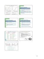
In this experimental context, it has been observed (Slooff, 1983; Chapter 18)
that SSDs from tests of complex mixtures generally have steeper slopes than the
SSDs of the individual chemicals in the mixture (Figure 21.1). A probable cause is
that the single chemicals in a complex cocktail of contaminants not only act as
chemicals with a specific toxicity but also contribute to joint additive toxicity, when
they are present below their threshold concentration (Hermens and Leeuwangh,
1982; Verhaar et al., 1995). This is often referred to as baseline toxicity. The results
of the experimental study by Pedersen and Petersen (1996) seems to be in accordance
with this theory. They observed that the standard deviation of a set of toxicity data
for a set of five laboratory test species tended to decrease (i.e, the slope of the SSD,
plotted as a cumulative distribution function, or CDF, would increase) with an

increasing number of chemicals in the mixture, although the number of species in
these experiments was small compared to many SSDs or species in field communities.
The relationships between the calculated and measured msPAFs and between
these msPAFs and measures of community responses in the field are complicated

© 2002 by CRC Press LLC

and have not as yet been demonstrated clearly. Variance in the composition of the
mixture may lead to varying effects on communities, depending on the dominant
modes of action and the taxa present. Obviously, the relation between observed
toxicity and the toxicity of mixtures predicted with SSDs requires further develop-
ment of concepts and technical approaches, to yield outcomes beyond the level of
relative measures of risks (Chapter 22).

21.1.3 P

ROBABILITY



OF

E

FFECTS



FROM

SSD

S

The criteria generated from SSDs and the risks estimated from SSDs (PAFs or PESs)
are often described as probabilistic without defining an endpoint that is a probability
(Suter, 1998a,b). This issue relates to the problem discussed above that the users of
SSDs often do not clearly define what they are estimating when they use SSDs. The
issue becomes important when communicating SSD-based results to risk managers
or other interested parties.
When SSDs are used as models of the PES for an individual species, the
sensitivity of the species is treated as a random variable. The species that is the
assessment endpoint is assumed to be a random draw from the same population of
species as the test species used to estimate the distribution (Van Straalen, 1990;
Suter, 1993). The output of the model is evidently probabilistic, namely, an estimate
of the PES on the endpoint species. For example, the probability of toxic effects on
rainbow dace given an ambient concentration in a water body may be estimated
from the distribution of the sensitivity of tested fish. As with the use of SSDs as
models of communities (i.e., to calculate PAFs), uncertainties and variability are
associated with estimating a PES. Given the parameter uncertainty due to sampling

FIGURE 21.1

SSDs for single compounds and a large mixture, showing the steepness (

β

)
of the CDF for the large mixture as compared to individual compounds. (Based on data from
De Zwart, Chapters 8 and 18.)

0
0.1
0.2
0.3
0.4
0.5
0.6
0.7
0.8
0.9
1
-2.5 -2 -1.5 -1 -0.5 0 0.5 1 1.5 2 2.5
Log
10
Toxic Units
Complex mixture,

β
= 0.17
Nonpolar Narcotics,

β
= 0.39
Organophosphates,

β
= 0.71
Potentially Affected Fraction

© 2002 by CRC Press LLC

and sample size, a confidence interval for the PES can be calculated (Chapters 5
and 17; Aldenberg and Jaworska, 2000). That is, one could calculate the probability
that the PES is as high as

P

z

. However, at present, none of the standard SSD-based
assessment methods claims to estimate risks to individual species.
More commonly, SSDs are used to generate output that is not a probability. That
is, when calculating HC

p

,

p

is the proportion of the community that is affected, not
a probability

.

Similarly, when calculating a PAF, the

F

is a fraction (or equivalently,

a proportion) of the community affected, not a probability. If we estimate the
distributions of these proportions, then we can estimate the probability of a pre-
scribed proportion. Hence, one could estimate the probability that the PAF is a high
as

F

x

or the HC

p

is as low as

C

y

given variance among biotic communities, uncertainty
due to model fitting, or any other source of variability or uncertainty. Parkhurst et al.
(1996) describe a method to calculate the probability that the PAF is as large as

F

x

at a specified concentration given the uncertainty due to model fitting. The calculation
of confidence intervals on HC

p

to calculate conservative criteria is conceptually
equivalent (Van Straalen and Denneman, 1989; Aldenberg and Slob, 1993).
The practical implications of this become apparent when considering the need
to explain clearly the results of risk assessments to decision makers and interested
parties (Suter, 1998b). One must explain that the probabilities resulting from various
SSD-based methods are probabilities of some event with respect to some source of
variance or uncertainty. In the explanation of SSD results, it should be clear that
there are various ways by which the SSD approach may analyze sources of uncer-
tainty and variability (see Chapters 4 and 5), and many sources that may be included
or excluded. Hence, risk assessors should be clear in their own minds and in their
writings concerning the endpoint that they intend to convey.

21.2 STATISTICAL MODEL ISSUES
21.2.1 S

ELECTION



OF

D

ISTRIBUTION

F

UNCTIONS

AND

G

OODNESS

-

OF

-F

IT

The choice of distribution functions has been the subject of much debate in published
critiques of the use of SSDs. Smith and Cairns (1993) objected to the fact that there
is no good basis for selecting a distribution function when, as is often the case, the
number of observations is small. Many users of SSDs simply employ a standard
distribution that has been chosen earlier by a regulatory agency or by the founders
of their preferred assessment method. This can lead to SSDs that badly fit the data.
See, for example, Figure 21.2, or Aldenberg and Jaworska (1999). Although the use
of a standard model can be defended as easy, consistent, and equitable, poor fits
cast doubt on the appropriateness of the method. There are various alternatives for
selecting distribution functions.
First, a chosen function may be considered acceptable based on failure to reject
the null hypothesis that the distribution of the data is the same as the distribution
defined by the function. Fox (1999) correctly raised the objection to this criterion

that failure to reject the null hypothesis does not mean that the function is a good
fit to the data. Statistical inference does not allow one to accept a null hypothesis
based on failure to reject.

© 2002 by CRC Press LLC

Second, it is preferable to choose functions based on goodness-of-fit or other
statistical comparisons of alternative functions, rather than by testing hypotheses
concerning a chosen function. Versteeg et al. (1999) used this approach, fitting the
uniform, normal, logistic, extreme value, and exponential distributions to 14 data
sets. Hoekstra et al.



(1994) compared lognormal and log-logistic fits to data for
26 substances and found that the lognormal was consistently preferable. However,
Van Leeuwen (1990) pointed out that the demonstrations of good fits of the log
logistic are based on relatively large sets of acute LC

50

and EC

50

values. The much
more heterogeneous chronic NOEC data sets may not have the same distribution
and usually do not provide enough observations to evaluate the fit rigorously. The
method for calculating water quality guidelines for trigger values in Australia and
New Zealand specifies selecting a distribution function from the Burr family based

on goodness-of-fit analyses (ANZECC, 2000).
Third, functions may be selected based on their inherent properties rather than
their fit to the data. In this respect, statistical arguments have been used more
frequently than ecological arguments. Aldenberg and Slob (1993) chose the logistic
because it is more conservative than the normal distribution (generates lower HC

5

values), and because it is more computationally tractable. Fox (1999) objected that
mathematical tractability is not an appropriate basis for choosing a function. Alden-
berg and Jaworska (1999) suggested a bimodal function to address misfits caused
by bimodality of the data set, which are in turn caused by the inclusion of subgroups
of sensitive and insensitive species. Fox (1999) and Shao (2000) argued for the three-
parameter Burr type III function, of which the logistic is a special case, because the
additional parameter provides greater flexibility. However, for both approaches, the
estimation of additional parameters enhances concerns with small sample sizes.
Wagner and Løkke (1991) preferred the normal distribution based on its central

FIGURE 21.2

A probit function (linearized lognormal) fit to freshwater acute toxicity data
for tributyltin. (From Hall, L. W., Jr. et al.,

Human and Ecological Risk Assessment,

6(1),
141, 2000. With permission.)
99
90
70

50
30
10
1
10
2
10
3
10
4
10
5
10
6
10
7
10
8
TBT Concentration (ng/l)
Percentile Rank Sensitivity

© 2002 by CRC Press LLC

position in statistics, promising wide applicability. Aldenberg and Jaworska (2000)
supported that argument. However, it was recognized early in the development of
SSDs that many data sets are not fit well by normal or lognormal distributions
(Erickson and Stephan, 1985). The U.S. EPA used the log-triangular distribution
because of its good fit (particularly with its truncated data sets) and its form, which
is consistent with the biological fact that there are no infinitely sensitive or insensitive
species (U.S. EPA, 1985a). Some use empirical distributions because they do not

require assumptions about the true distribution of the data (Jagoe and Newman,
1997; Giesy et al., 1999; Newman et al., 2000; Van der Hoeven, 2001). Others have
used empirical distributions as a way to display the observed distribution of species
sensitivities when neither PAFs nor HC

p

values are calculated (Suter et al., 1999),
when a simple method is desired for early tiers of assessments (Parkhurst et al.,
1996), or when none of the parametric distributions is appropriate (Newman et al.,
2000). The use of linear interpolation to calculate HC

p

values is equivalent to the
use of an empirical distribution.
Finally, knowledge of the chemical may guide the choice of model. For example,
specifically acting chemicals will tend to have large variances and asymmetry due
to extremely sensitive or insensitive species (Vaal et al., 1997). If it is not possible
to partition the data sets for such chemicals (Section 21.5.5), it may be wise to use
empirical distributions rather than symmetrical functions.
Some have argued that the choice of function makes little difference, because
the numerical results are similar in many cases. An OECD workshop compared the
lognormal, log-logistic, and log-triangular distributions and concluded that the dif-
ferences in the HC

5

values were insignificant (OECD, 1992). Smith and Cairns
(1993) also stated that those distributions give relatively similar results. Fox (1999)

argued that the choice of function matters, based on his demonstration that adding
a parameter can make “up to a 3-fold difference.” Newman et al. (2000) argued that
the use of parametric functions is a mistake, because they often fail to fit real data
sets. Therefore, they stated that empirical distributions fit to data by bootstrapping
should be preferred to avoid indefensible assumptions. Others have argued that this
practice is defensible only for large sample sizes (Van der Hoeven, 2001). Also, the
use of parametric models is more suited to extensions of the extrapolation model,
such as the addition of variation in bioavailability or biochemical parameters related
to partitioning (Aldenberg and Jaworska, 2000; Van Wezel et al., 2000).
An issue that is likely to be more important for the numerical outcome than the
choice of model is the related issue of data pretreatment discussed in Section 21.5.
The choices made in data treatment, often related to ecological issues, can influence
model choice and output precision; therefore, the debate should not focus solely on
statistical concerns.

21.2.2 C

ONFIDENCE

L

EVELS

EQC may be based on protecting a percentage of species or protecting a percentage
with prescribed confidence. An example of the former practice is that the U.S. EPA
has used the HC

5

without uncertainty estimates to calculate criteria (U.S. EPA,

1985a; Chapter 11). Examples of the latter are Kooijman (1987), who developed

© 2002 by CRC Press LLC

factors to protect all members of a community with 95% confidence, and Van
Straalen and Denneman (1989) and Aldenberg and Slob (1993), who developed
factors to protect 95% of species with 95% confidence. Wagner and Løkke (1991)
also developed a method for protecting 95% of species with 95% confidence and
showed that the confidence intervals of HC

p

values are similar to what are called
“tolerance limits” in distribution-based techniques for quality control of industrial
products.
Suter (1993) pointed out that the those calculations are incomplete analyses of
uncertainty concerning the HC

p

. They account for uncertainty due to fitting a function
to a sample but not due to uncertainties in the individual observations including
extrapolations from the test endpoints to the values to be protected and systematic
biases in the test data sets.
Van Leeuwen (1990) argued that the use of lower 95% confidence bounds,
particularly when

n

is low, leads to unrealistically low values (Figure 21.3). However,

the use of confidence bounds on the HC

p

is still advocated as a prudent response to
the uncertainties in the method (Newman et al., 2000), and confidence bounds are
now routinely reported when calculating HC

p

values in the Netherlands (Verbruggen
et al., 2001).
The issue of whether to use confidence intervals is also important in the context
of risk assessment (see Figure 21.3). The use of confidence intervals may be limited
by the presentation method, as in the case of spatial mapping of PAF values
(Chapters 16 and 19). There is also a theoretical objection. Solomon and Takacs
(Chapter 15) argue that the use of confidence intervals on SSDs is inadvisable unless

FIGURE 21.3

A graphical representation of confidence bounds for the HC

5

and the PAF.
The figure shows the 5 and 95% confidence limits of

10

log(HC

5

) and the 5th, 50th, and 95th
percentiles of the PAF. Dots represent toxicity test results. (Courtesy of Tom Aldenberg.)
Range PAF
-1 -0.8 -0.6 -0.4 -0.2 0
0
0.05
0.1
0.15
0.2
10
Log Concentration (mg/l)
Potentially Affected Fraction
Range
10
Log(HC
5
)

© 2002 by CRC Press LLC

important species can be weighted, because the use of confidence intervals assumes
that all species are equal in the sense of their roles and functions in the ecosystem
and that they can be treated in a purely numerical fashion. That objection is applicable
to any use of SSDs, with or without uncertainty analysis. In practice, accounting
for uncertainties concerning predicted effects is desirable, both to improve the basis
for decision making and for the sake of transparency concerning the reliability of
results. Thus, the context of the application and the preferences of the decision maker

may limit or promote the reporting of confidence intervals or probabilities of pre-
scribed PAF or PES levels. In any case, it is important to specify what sources of
uncertainty are included in the calculation.

21.2.3 C

ENSORING



AND

T

RUNCATION

Because of the symmetry of most of the distribution functions used in SSDs, asym-
metries in the data can affect the results in unintended ways. In particular, even after
log conversion, many ecotoxicological data sets contain long upper tails due to highly
resistant species (see, e.g., Figure 21.2). If these data are used in fitting the distri-
bution, the fitted 5th percentile can be well below the empirical 5th percentile.
One approach to eliminating this bias is to censor the values for the highly
resistant species, as recommended by Twining and Cameron (1997). To avoid both
the bias and the apparent arbitrariness of censoring, the U.S. EPA simply truncates
the distribution when calculating risk limits (U.S. EPA, 1985a; Chapter 11). That is,
all data are retained, but only the lower end of the distribution is fit. This, however,
can lead to a misfit to the total data set, as shown by Roman et al. (1999). Hence,
its use is limited to the calculation of criteria, as in U.S. EPA (1985a), or to risk
assessments with low PAFs.
Another approach is to analyze the data set by fitting mixed (i.e., polymodal)

models to generate risk limits. Aldenberg and Jaworska (1999) applied a bimodal-
normal model to the (log) toxicity data to this end. The parameter estimates were
generated through Bayesian statistics and provide estimates for the HC

p

for the most
sensitive group of species, independent of prior knowledge about sensitive species.
This practice can eliminate the need for censoring or truncating but is computation-
ally intensive (Aldenberg and Jaworska, 1999). Shao (2000) used a mixed Burr
type III function for the same purpose.
Pretreatment of data may reduce the need for censoring or truncation by reducing
biases in data sets due to differences in bioavailability or other confounding factors
(Section 21.5). Fitting alternative models may also remove the need for censoring
and truncation.

21.2.4 V

ARIANCE

S

TRUCTURE

Smith and Cairns (1993) point out that the data sets used in SSDs are likely to
violate the assumption of homogeneity of variance. That is, test results from different
laboratories using different test protocols are likely to have different variances. They
recommend the use of weighting to achieve approximate homogeneity.

© 2002 by CRC Press LLC

21.3 THE USE OF LABORATORY TOXICITY DATA

SSDs are derived from single-species laboratory toxicity data. Some of the criticisms
of SSDs are actually criticisms of any use of those data, and pertain also to other
approaches, such as the application of safety factors. These issues will be discussed
only briefly here, because they are not peculiar to SSDs.

21.3.1 T

EST

E

NDPOINTS

SSDs are most often distributions of conventional single-species toxicity test end-
points, and the HC

p

values and other values derived from them can be no better than
those input values. All of the conventional test endpoints have some undesirable
properties (Smith and Cairns, 1993), but whether these are serious depends on the
context of SSD application. Furthermore, the appropriateness of test endpoints
cannot be fully judged until their relationships to the assessment endpoints are
clarified.
LC

50

values represent severe effects that are unlikely to be acceptable in regu-
latory applications of SSDs to derive quality criteria for routine exposures. However,
they may be properly applied in assessments of short-term exposures, as in spills or
upsets in treatment operations.
No-observed-effect concentrations (NOECs) and lowest-observed-effect concen-
trations (LOECs) have all of the problems of test endpoints that represent statistically
significant rather than biologically or societally significant effects. In particular, they
do not represent any particular type or level of effect, so distributions of NOECs or
LOECs are distributions of no specific effect (Van Leeuwen, 1990; Van der Hoeven,
1994; Laskowski, 1995; Suter, 1996). NOECs are particularly problematical because
they may be far below an actual effects level or may correspond to relatively large
effects, which are not statistically significant because of high variance and low
replication (Van der Hoeven, 1998; Fox, 1999). Wagner and Løkke (1991) recognized
these problems, but used NOECs anyway as the best available option to derive EQCs.
Van Straalen and Denneman (1989) argued that NOECs are reasonably representative
of effects thresholds in the field. They recommend using only NOECs for reproduc-
tive effects to derive criteria, both to increase consistency and because of the impor-
tance and sensitivity of reproduction.
The relationship between SSDs and ecosystem processes has been an issue of
debate. Smith and Cairns (1993) argued that criteria based on SSDs do not protect
ecosystem functional responses, implying that such responses are likely to be more
sensitive than organismal responses. Hopkin (1993) argued that SSDs are unlikely
to protect ecosystem processes, because key processes may be dominated by a few
species, such as large earthworms, and those species may be more sensitive than
95% of species. Forbes and Forbes (1993) also suggested that SSDs do not address
ecosystem function, but they argued that ecosystem function is likely to be less
sensitive than structure, and therefore SSDs will be overprotective. Various authors
have stated in the context of pesticide risk assessment that ecosystem function is
likely to be less sensitive than organismal responses, because of functional redun-

dancy (Solomon, 1996; Solomon et al., 1996; Giesy et al., 1999). Neither these

© 2002 by CRC Press LLC

arguments from theory nor the attempts to confirm SSDs using mesocosm data
(Section 21.8.2) have resolved this issue. The appropriate resolution in particular
cases should depend on the assessment endpoints chosen.
One might respond to both sides by pointing out that SSDs, which are based
primarily, if not entirely, on tests of vertebrate and invertebrate animals, should not
be expected to estimate responses of ecosystem functions which, in aquatic systems,
are dominated by algae, bacteria, and other microbes. As a pragmatic solution,
Van Straalen and Denneman (1989) argue that, if ecosystem functions are of concern,
criteria should be derived using appropriate test endpoints. This pragmatic solution
was adopted by using terrestrial microbial functions for derivation of soil quality
criteria in the Netherlands. Distribution functions for data sets of microbial and
fungal processes and enzyme activities (Chapter 12), are used to derive FSDs
(function sensitivity distributions) and the lowest FSD or SSD is chosen to derive
the EQC (Figure 21.4). The Canadian approach in deriving EQCs applies another
pragmatic approach, using test endpoints that relate to the assessment problem
directly (Chapter 13).

21.3.2 L

ABORATORY



TO

F

IELD

E

XTRAPOLATION

From the beginning of the use of SSDs, the importance and difficulty of laboratory-
to-field extrapolation has been discussed (U.S. EPA, 1985a; Van Straalen and Den-
neman, 1989). Differences believed to be important include a range of phenomena
(see Chapter 9, Table 9.1), including bioavailability, spatial and temporal variance in

FIGURE 21.4

SSD and soil FSD for cadmium. (Data from Crommentuijn et al., 1997.)
10
-1
10
0
10
1
10
2
10
3
10
4
10
5
0

0.1
0.2
0.3
0.4
0.5
0.6
0.7
0.8
0.9
1
Cumulative density
Function NOECs
Fitted FSD
Species NOECs
Fitted SSD
Concentration (mg/kg standard soil)

© 2002 by CRC Press LLC

field exposures, and genetic or phenotypic adaptation. However, the issue of labo-
ratory-to-field extrapolation is another problem that is generic to laboratory toxicol-
ogy and not peculiar to SSDs. If the use of laboratory data cannot be avoided, due
to the lack of field data or problems with field–field extrapolation, the laboratory
data can be adjusted or pretreated with the aim to improve field relevance.
For example, concerning bioavailability, Smith and Cairns (1993) argued that
SSDs are inappropriate because environmental conditions, particularly water chem-
istry, do not necessarily match test conditions. However, test endpoints may be
adjusted for environmental chemistry, or exposure models may be used to estimate
bioavailable concentrations rather than total concentrations.
Data treatment cannot solve all extrapolation problems, because of the complex

nature of ecological phenomena. For example, genetic adaptation or pollution-
induced community tolerance may occur when populations or communities are
chronically exposed to contaminants. Field populations or communities may become
less sensitive due to evolved capabilities to physiologically exclude or sequester
contaminants or to compensate for effects, a phenomenon not addressed in laboratory
toxicity tests. Strong evidence has shown the existence of such responses upon
contaminant exposure (Posthuma et al., 1993; Rutgers et al., 1998). The occurrence
of genetic adaptation by sensitive species may cause reduced variance of sensitivities
in a community, which may lead to a “narrowed” SSD in the field, as observed by
Rutgers et al. (1998) (Figure 21.5).
The selection and treatment of input data for use in SSDs can address some
discrepancies between the laboratory and field, and various options are treated in
Sections 21.4 and 21.5. However, other discrepancies must be treated as sources of
uncertainty until they are resolved by additional research.

FIGURE 21.5

FSDs for microbial communities showing the reduced variance (increased
steepness of CDFs) for metal-tolerant communities. Tolerance was measured using activity
measurements of sampled microbial communities on Biolog™ plates. Microbial tolerance
increases with decreasing distance from a former zinc smelter and with increasing soil zinc
concentrations. (Courtesy of M. Rutgers.)
0
0.2
0.4
0.6
0.8
1
0.01 0.1 1 10 100 1,000 10,000
Sensitivities of breakdown functions

(EC
50
Biolog
in mg Zn/l)
Frequency of sensitivities
(cumulative)
20 km (14 mg Zn/kg soil)
14 km (35 mg Zn/kg soil)
6 km (83 mg Zn/kg soil)
2 km (104 mg Zn/kg soil)
1 km (364 mg Zn/kg soil)
Field soil characteristics

© 2002 by CRC Press LLC

21.4 SELECTION OF INPUT DATA

The dependence of SSDs on the amount and quality of available data has been
particularly obvious to critics. This section discusses issues of data selection and
adequacy.

21.4.1 SSD

S



FOR

D

IFFERENT

M

EDIA

EQC are set for specific compartments: water, air, soil or sediment in different
countries (Chapters 10 through 14). To this end, specific SSDs are constructed from
data of terrestrial, aquatic, or benthic species. However, complications arise when
associating SSDs with media.
The U.S. EPA and other environmental agencies have routinely derived separate
freshwater and saltwater criteria (U.S. EPA, 1985a). Because the toxicity of some
chemicals is not significantly influenced by salinity (Van Wezel, 1998), that distinc-
tion is not always necessary (Chapter 15). In particular, the U.S. EPA combines
freshwater with saltwater species for neutral organic chemicals (U.S. EPA, 1993).
The Dutch RIVM combines saltwater and freshwater data if no statistical significant
difference can be demonstrated. Solomon et al. (2001) combined freshwater and
saltwater data, unless the intercept or slope of the probit SSD models was different.
The assignment of species to a medium may be unrealistic, since some species
are exposed through various environmental compartments, either during their whole
life cycle (e.g., a mammal that drinks water and feeds from terrestrial food webs)
or during parts thereof (amphibians). This may pose specific problems related to
combining different species in an SSD and the use of one species in SSDs for more
than one compartment. When species are significantly exposed through several
compartments, SSDs can be based on total dose received by those species rather
than ambient concentrations. Subsequently, given the SSD, criteria for the different
environmental compartments can be calculated using a multimedia model (e.g.,
Mackay, 1991) to calculate critical concentrations in the relevant environmental
compartments. When both direct and food chain exposure exists in a species assem-

blage, they can be combined by relating the food chain exposure to concentrations
in a common exposure compartment such as water or sediment by using bioconcen-
tration factors (BCFs) or biota-to-sediment accumulation factors (BSAFs)
(Chapter 12). When species with multiple exposure routes are omitted or when
exposure routes are ignored, results may be biased.
An alternative solution to the problem of complex exposures is to use body
burdens as exposure metrics (McCarty and Mackay, 1993). That is, the SSD would
be distributed relative to concentration of the chemical in organisms rather than in
an ambient medium. This approach would be expected to yield lower variances
among species. It would be particularly useful for risk assessments of contaminated
sites.
Problems also arise when media have multiple distinct phases. In particular,
sediment contains aqueous and solid phases, and soil contains aqueous, solid, and
gaseous phases. This problem is addressed by assuming a single dominant exposure
medium such as sediment pore water, so the exposure axis of the SSD is simply

© 2002 by CRC Press LLC

taken as the concentration in water (e.g., Chapter 12). However, equilibrium assump-
tions may not hold, and these cases may also need to be treated as multimedia
exposures resulting in a combined dose.

21.4.2 T

YPES



OF

D

ATA

A fundamental problem of SSDs is defining the range of test data that is appropriate
to a model and to an environmental problem. If SSDs are interpreted as models of
variance in species sensitivity, it is necessary to minimize other sources of variance.
These sources of extraneous variance potentially include variance in test methods,
test performance, properties of test media, and test endpoints. This consideration
has led to specification of acceptable types of input data as in the U.S. EPA procedure
for deriving EQC (U.S. EPA, 1985a; Chapter 11).
Rather than eliminating or minimizing extraneous variance, sources of variance
may be explicitly acknowledged as part of the SSD methodology. For example, in
deriving soil screening benchmarks, Efroymson et al. (1997a,b) recognized that
variance in test soils was significant, so they considered their distributions to be
distributions of species/soil combinations (see also Section 21.5.1). Such inclusive-
ness can quickly carry us beyond the topic of SSDs. For example, in setting bench-
mark values for sediments, various laboratory and field tests and field observations
of organisms, populations, and communities have been combined into common
distributions that are difficult to characterize (Long et al., 1995; MacDonald et al.,
1996). It may well be that SSDs for soil will almost always have other sources of
variance that are large relative to the variance among species, with or without
provisional correction for bioavailability. In that sense, SSD results become part of
a multivariate description, in which the species sensitivities are one of the descriptor
variables and pH, etc. are others. This multivariate approach has been taken in
modeling effects of multiple stressors on plants (Chapter 16).
The selection of data with consistent test endpoints may be difficult. As discussed
above (Section 21.3.1) test endpoints based on statistical hypothesis testing are
inherently heterogeneous. Hence, SSDs based on NOECs, LOECs, or CVs contain
variance due to differences in the response parameter and the level of effect. Con-

ceivably, one could select data to minimize this variance. For example, one could
use only NOECs that are based on reproductive effects and that do not cause more
than a 10% reduction in fecundity. However, that is not part of current practice.
SSDs are models of the variance among species, so species should be selected
that are of concern individually or as members of communities. For example, algae
and microbes are usually valued for the functions they perform and not as species.
Therefore, the exclusion of algae and microbes from SSDs, as in the U.S. EPA
method, may be appropriate (U.S. EPA, 1985a).
In contrast to these concerns, Niederlehner et al. (1986) suggested that the
selection of species may not matter. Based on a study of cadmium, they argue that
the loss of 5% of protozoan species in a test of protozoan communities on foam
substrates is equivalent to the U.S. EPA HC
5
, which is derived from tests of diverse
fish and invertebrates. However, it seems advisable to choose species based on their
© 2002 by CRC Press LLC
susceptibility to the chemical, particularly when assessing compounds with specific
modes of action such as herbicides or insecticides, and on whether they represent
the endpoint of concern.
21.4.3 DATA QUALITY
The issue of data quality has received considerable attention in frameworks to derive
quality criteria. This is because the use of data sets that have not been quality assured
can introduce extraneous variance into SSDs, and can introduce biases into SSD
models. The U.S. EPA has specified quality criteria for the data used to derive water
quality criteria (U.S. EPA, 1985a). Emans et al. (1993) used OECD guidelines for
toxicity tests to qualify data for their study. The aquatic ECOFRAM used quality
criteria from the Great Lakes Initiative (U.S. EPA, 1995). In the Netherlands, all
data used for derivation of quality criteria for water, soil, or sediment with SSDs
are evaluated according to a quality management test protocol that is continuously
updated (Traas, 2001).

Some SSD studies apparently accept all available data, with unknown effects on
their results. It has been argued that all available data should be used because variance
among species is large relative to variance among tests (Klapow and Lewis, 1979). It
should be noted in this respect that the readily accessible databases usually have some
degree of quality control on the input data, and this quality control applies indirectly
to the SSDs derived from them. However, quality control is needed even when using
generally accepted databases. After merging data from various databases, De Zwart
(Chapter 8) applied an extensive quality control prior to using the merged data set.
This was not based on quality checks to all original references (>100,000), but on
removal of double entries and a check for false entries based on pattern recognition.
Whatever the application, explicit and well-described data quality procedures improve
transparency and repeatability of an analysis as well as the reliability of the results.
21.4.4 ADEQUATE NUMBER OF OBSERVATIONS
In the derivation of environmental quality criteria, various requirements have been
suggested regarding the adequate number of observations based on differing toler-
ances for uncertainty concerning the HC
p
(Figure 21.6). The smallest data require-
ment (n > 3) was specified by early Dutch methods (Van de Meent and Toet, 1992;
Aldenberg and Slob, 1993). Van Leeuwen (1990) indicated that five species would
be adequate based on uncertainty and ethical and financial considerations. Danish
soil quality criteria also require a minimum of five species (Chapter 14). The U.S.
EPA method requires at least eight species from different families and a prescribed
distribution across taxa (U.S. EPA, 1985a; Chapter 11).
Various suggestions for adequate numbers have been given for SSDs used in
ecological risk assessments, based on statistical and ecological grounds. The method
applied by the Water Environmental Research Foundation in the United States does
not specify a minimum n, but the authors indicate that the eight chronic values for
zinc were too few, while the 14 values for cadmium were sufficient (Parkhurst et al.,
© 2002 by CRC Press LLC

1996). Four chronic or eight acute values were required by the Aquatic Risk Assess-
ment and Mitigation Dialog Group (Baker et al., 1994). Cowan et al. (1995) stated
that SSDs may be useful when more than 20 species have been tested, because that
number is required to verify the form of the distribution. Newman et al. (2000)
estimated that the optimal number of values in an SSD is 30, the median number
needed to approach the point of minimal variation in the HC
5
. Vega et al. (1999)
and Roman et al. (1999) conclude that, for logistically distributed data, this point is
approached when ten or more values are available.
De Zwart (Chapter 8) presented evidence that the shape of the SSD (the slope)
was associated with the TMoA of the compound. Given the idea of such an intrinsic
(mode-of-action related) shape parameters for SSDs, he found that the number of
test data needed to obtain the required value of the shape parameter for a certain
compound would range from 25 to 50. However, due to the observed mode-of-
action-related patterns among shape parameters for different compounds, it was
suggested that the use of surrogate shape values, derived from data of compounds
with the same TMoA, could solve the problem of data limitation. Estimation of the
position parameter requires far fewer data than estimation of the slope.
Apparently, there are numbers, beyond which the SSD does not change consid-
erably in shape or estimated parameters. Aldenberg and Jaworska (2000) gave
relationships for confidence limits related only to the number of input data. For
example, at n = 4, the estimated HC
5
is rather imprecise, with a 90% confidence
interval between 0.07 and 37%. This means that the median HC
5
derived from this
low number of data is very often not protective of the fraction of species specified
as being protected in as many as 37% of cases (secondary risk). If decision makers

FIGURE 21.6 Confidence intervals for SSDs based on the normal distribution, depending
on the number of data only. The lines show the median and 5th to 95th percentiles of the
PAF for n = 10 and n = 30. (The figure was kindly prepared by T. Aldenberg according to
Aldenberg and Jaworska, 2000.)
-3 -2 -1 0 1 2 3
0
0.1
0.2
0.3
0.4
0.5
0.6
0.7
0.8
0.9
1
Standardized
10
Log (Concentration)
Potentially Affected Fraction
Confidence limits for n = 10
Confidence limits for n = 30
© 2002 by CRC Press LLC
want to be more certain that 95% of the species are protected, upper confidence
limits can be calculated from the known patterns (e.g., n = 8), where the upper
confidence limit of the HC
5
falls below 25%.
When data are in short supply, as is the case for many substances, an optimum
number of observations will not be reached. With such limitations, decision makers

can either ask for estimated HC
p
values with specified confidence, or for specification
of the uncertainty in the ecological risk assessment.
21.4.5 BIAS IN DATA SELECTION
The species used for toxicity testing are not a random sample from the community
of species to be protected (Cairns and Niederlehner, 1987; Forbes and Forbes, 1993).
This nonrandomness can potentially bias the SSDs. However, the magnitude and
direction of the bias are not clear.
One argument is that species are selected for their sensitivity, and therefore SSDs
have a conservative bias (Smith and Cairns, 1993; Twining and Cameron, 1997). In
the United States, the validity of this argument is supported by the fact that the
U.S. EPA defined its base data set to ensure the inclusion of taxa that were believed
to be sensitive (U.S. EPA, 1985a). The ARAMDG recommended choosing species
at “the sensitive region of the distribution” (Baker et al., 1994). Further, for biocides,
testing may be focused on species that are closely related to the target species and
therefore likely to be sensitive. An OECD workshop concluded that, in general, this
bias is not unreasonable (OECD, 1992). However, there is little basis for this
conclusion beyond expert judgment.
Another source of bias in data selection is the narrow range of taxa tested relative
to the range of taxa potentially exposed (Smith and Cairns, 1993). For example,
aquatic toxicity testing has focused on fish and arthropods and has tended to neglect
other vertebrate and invertebrate taxa. Algal and microbial taxa are almost inevitably
underrepresented when SSDs are intended to include them. Toxicity testing of birds
has focused on the economically important Galliformes and Anseriformes rather
than the much more abundant Passeriformes. In addition, species from some com-
munities such as deserts tend to be underrepresented (Van der Valk, 1997). These
biases will tend to reduce the variance of the SSD, which could cause an anticon-
servative bias in estimates of low percentiles.
21.4.6 USE OF ESTIMATED VALUES

Toxicity data estimated from models have been used in cases where the available
test data are not sufficiently numerous to derive an SSD. Models have been developed
for compound-to-compound, SSD-to-SSD, or species-to-species extrapolation.
Models may be used for compound-to-compound extrapolation. Van Leeuwen
et al. (1992) assembled a set of 19 quantitative structure–activity relationships
(QSARs) that estimate NOECs for chemicals with a baseline narcotic TMoA.
Because all of their QSARs used the octanol–water partitioning coefficient (K
ow
) as
the independent variable, it was possible for the authors to derive a formula for
estimating the HC
5
for any narcotic chemical from its K
ow
. If any test data were
© 2002 by CRC Press LLC
available, they could be used along with the QSAR-derived values in an SSD. The
same approach could be used to supplement any data set when an appropriate QSAR
is available. However, the use of QSARs adds additional uncertainties due to impre-
cision of the model and the potential for misclassification of the chemical. The
QSAR model is also the average fit to the individual toxicity data, thereby possibly
reducing the variance of the SSDs compared to the original data. DiToro et al. (2000)
used a similar approach to estimate the HC
5
for polycyclic aromatic hydrocarbon
(PAHs) from K
ow
and a QSAR for narcosis.
SSDs have also been approximated for small numbers of species by using
properties of SSDs derived from large data sets. One approach is to assume that the

mean and standard deviation are independent (Chapter 8; Luttik and Aldenberg,
1997). One may then derive a SSD from a mean estimated from the small set of
test endpoints for the chemical of concern and a pooled variance derived from several
SSDs for the same class of chemicals. Alternatively, one may use resampling of
small data sets from large sets used to derive HC
p
values, calculate the quotients of
the lowest endpoint in the samples to the HC
p
for that chemical, and derive a
distribution of that ratio for each small n (Host et al., 1995). These approximations
introduce another source of uncertainty to the use of SSDs, so the authors of both
methods recommend conservative estimates of the HC
p
. Alternatively, when few
chronic data are available, one may approximate the chronic SSD by applying an
acute-to-chronic ratio to the acute SSD (Section 8.5.2).
SSDs have been supplemented by using models to extrapolate from a small set
of test species to a larger set of species of interest. Traas et al. (Chapter 19) used
this approach to derive SSDs for avian and mammalian wildlife from small sets of
avian and mammalian toxicity data. Their extrapolation models were based on
differences in dietary composition and intake rates among species. For animals
exposed through their diet, the exposure component of sensitivity is difficult to
separate from the intrinsic toxicity of chemicals, unless based on concentrations in
target sites. These models are thus more based on exposure distributions than on
intrinsic toxicity distributions. However, other interspecies extrapolation models
could also serve that purpose.
Extrapolation models used in the construction of an SSD introduce additional
uncertainties. In particular, if they do not incorporate all of the relevant sources of
variance among species, they will tend to overestimate HC

p
values (i.e., be less
protective) when p is small.
21.5 TREATMENT OF INPUT DATA
Some of the limitations of, and objections to, SSDs may be addressed by processing
the data prior to calculation of the SSD. There are two possibilities for this. First,
processing changes the data with the same factor(s) for all species, for example, by
using a fixed factor correcting for differences in exposure between laboratory and
field (e.g., Traas et al., 1996). This shifts the distribution on the log-concentration
axis. Second, processing may consist of applying different factors for different
species, so that the variance of the data changes. Preprocessing of data is usually
done to improve the association of the SSD with the assessment endpoint. This
© 2002 by CRC Press LLC
may lead to better predictions of effects and may reduce one of the main problems
with the verification studies of SSDs, the dissimilarity of variances between SSDs
in the laboratory and in the field.
21.5.1 HETEROGENEITY OF MEDIA
The most common preprocessing of input data is normalization to reduce variance
among tests due to the physicochemical properties of the test medium. Those prop-
erties may influence the biological availability or toxicity of the compound.
Preprocessing of data is done for several metals, ammonia, and phenols in the
U.S. EPA water quality criteria (U.S. EPA, 1985a). In the Netherlands, metal con-
centrations in soil are adjusted for soil chemistry (Van Straalen and Denneman,
1989). Variables used have included pH, hardness, temperature, clay content, and
organic matter content. In the Netherlands, empirical formulae have been derived
by fitting a statistical function to sets of data that include the range of chemical
conditions encountered in the field. For example, normalization of metal concentra-
tions to a standard soil (with a fixed percentage organic matter and clay) is applied,
by using regression equations that relate metal contents to soil properties for a range
of relevant areas (Lexmond and Edelman, 1986). These equations are routinely used

in normalizing laboratory toxicity data to a so-called standard soil. After normaliza-
tion, an SSD is made for the standard soil, and the EQCs for metals are derived
accordingly (Chapter 12). In applying these EQCs to field soils, the regression
equations are used inversely, so that a certain degree of site specificity is created in
the EQCs. As a secondary use of the empirical formulae, one can calculate whether
exceedence of EQCs will occur in case of changing substrate characteristics. For
example, Van Straalen and Bergema (1995) tested the expectation that soils will
become more acidic when normal agricultural practice ceases and therefore more
toxic due to the heavy metal load already present.
The proposed formulae are intended to normalize data to a standard chemistry,
so that the SSD does not contain extraneous variance. U.S. water quality criteria
and Dutch EQCs are adapted to local conditions by adjusting for the chemistry of
local media. They may be used to adjust the HC
p
or the entire distribution for local
conditions when performing a site-specific risk assessment (Hall et al., 1998). Stan-
dardization algorithms are important but are a source of debate in the use of SSDs.
They should at least be verified for their intended purpose, reducing the extraneous
variance in SSDs or improving the accuracy of site-specific assessments.
21.5.2 ACUTE–CHRONIC EXTRAPOLATIONS
For many chemicals, the available data are primarily acute, whereas regulators and
assessors are primarily concerned with chronic effects. Usually, there are insufficient
chronic test data to derive a chronic SSD.
The simplest option to fill this gap is to use a generic acute–chronic ratio to
convert the acute values to estimated chronic values. For example, De Zwart and
Sterkenburg (Chapter 18) used a factor of 10 and the Danish method uses a factor
of 3 (Chapter 14).
© 2002 by CRC Press LLC
Alternatively, the extrapolation factor may be chemical specific. When there are
not enough data to derive a chronic SSD, the U.S. EPA derives a chemical-specific

acute–chronic ratio (U.S. EPA, 1985a). The Water Environment Research Foundation
method uses acute–chronic ratios to estimate chronic SSDs, even when, as for copper
and zinc, a relatively large number of chronic values are available to derive a chronic
distribution directly (Parkhurst et al., 1996). Although the latter method allows for
direct derivation of chronic SSDs, in practice the authors prefer the SSDs obtained
from the larger number of acute values and assume that the use of acute SSDs and
acute–chronic ratios to estimate chronic SSDs does not increase uncertainty.
A further alternative, based on a different assessment of the acute–chronic
pattern, makes use of whole SSDs. The chapter on SSD regularities (Chapter 8) has
shown that the uncertainty of acute–chronic ratios for specific TMoAs can be
calculated from SSD parameters for chemicals with the same TMoA. This uncer-
tainty can then be combined analytically with that of the SSD itself. This uncertainty
is, however, of a quite different magnitude than acute–chronic ratios derived directly
from acute–chronic pairs for species, which also has consequences for further sta-
tistical properties (e.g., calculation of confidence intervals).
21.5.3 COMBINING DATA FOR A SPECIES
Often, more than one value will be available for a particular chemical, species, and
test endpoint. In such cases, it is generally desirable to reduce those multiple values
to a single observation.
For effects-based test endpoints where the test endpoint is clear (such as with
LC
50
values) and test conditions do not significantly differ, one may choose one of
the tests or average them. Selection might be based on the quality of the tests, the
magnitude of the result (e.g., choose the lowest value), or their relevance to the
situation being assessed (e.g., similarity of test water chemistry to the site; Suter
et al., 1999). If all values are acceptable, they may be averaged. The U.S. EPA uses
geometric means (U.S. EPA, 1985a).
For test endpoints based on hypothesis testing (i.e., most chronic toxicity data),
there is the additional problem that the endpoints are usually not for the same

response, the same level of response, or the same test conditions, so that averaging
is generally not appropriate. In such cases, the lowest value is commonly used
(Okkerman et al., 1991; Aldenberg and Slob, 1993). Van de Meent et al. (1990)
proposed using the lowest value when the test endpoint responses are different and
the geometric mean when they are the same. Such decisions can bias SSDs.
21.5.4 COMBINING DATA ACROSS SPECIES
In the use of SSDs, it is implicitly assumed that a set of tested species represents
independent observations from a random distribution. However, the variance in
sensitivity among species is not random. In particular, the responses of species that
are closely related taxonomically are more highly correlated than those distantly
related (Suter et al., 1983; LeBlanc, 1984; Slooff et al., 1986; Suter and Rosen, 1988;