Statistical Tools for Environmental Quality Measurement - Chapter 7 ppt

C H A P T E R 7
Tools for the Analysis of Spatial Data
There is only one thing that can be considered to exhibit random behavior in
making a site assessment. That arises from the assumption adopted by risk assessors
that exposure is random. In the author’s experience there is nothing that would
support an assumption of a random distribution of elevated contaminant
concentration at any site. Quite the contrary, there is usually ample evidence to
logically support the presence of correlated concentrations as a function of the
measurement location. This speaks contrary to the usual assumption of a
“probabilistic model” underlying site measurement results. Isaaks and Srivastava
(1989) capture the situation as follows:
“In a probabilistic model, the available sample data are viewed
as the result of some random process. From the outset, it should
be clear that this model conflicts with reality. The processes that
actually do create an ore deposit, a petroleum reservoir, or a
hazardous waste site are certainly extremely complicated, and
our understanding of them may be so poor that their complexity
appears as random behavior to us, but this does not mean that
they are random; it simply means that we are ignorant.
Unfortunately, our ignorance does not excuse us from the
difficult task of making predictions about how apparently
random phenomena behave where we have not sampled them.”
We can reduce our ignorance if we employ statistical techniques that seek to
describe and take advantage of spatial correlation rather than ignore it as a
concession to statistical theory. How this is done is best described by example. The
following discusses one of those very few examples in which sufficient
measurement data are available to easily investigate and describe the spatial
correlation.
ABC Exotic Metals, Inc. produced a ferrocolumbium alloy from Brazilian ore in
the 1960s. The particular ore used contained thorium, and slight traces of uranium,
as an accessory metal. A thorium-bearing slag was a byproduct of the ore reduction

process. Much of this slag has been removed from the site. However, low
concentrations of thorium are present in slag mixed with surface soils remaining at
this site.
The plan for decommissioning of the site-specified criteria for release of the site
for unrestricted use. Release of the site for unrestricted use requires demonstration
that the total thorium concentration in soil is less than 10 picocuries per gram
(pCi/gm). The applicable NRC regulation also provides options for release with
restrictions on future uses of the site. These allow soil with concentrations greater
steqm-7.fm Page 163 Friday, August 8, 2003 8:19 AM
©2004 CRC Press LLC
than 10 pCi/gm to remain on the site in an engineered storage cell provided that
acceptable controls to limit radiation doses to individuals in the future are
implemented.
In order to facilitate evaluation of decommissioning alternatives and plan
decommissioning activities for the site, it was necessary to identify the location,
depth, and thickness of soil-slag areas containing total thorium, thorium 232 (Th
232
)
plus thorium 228 (Th
228
), concentrations greater than 10 pCi/gm. Because there are
several possible options for the decommissioning of this site, it is desirable to
identify the location and estimated volumes of soil for a range of total thorium
concentrations. These concentrations are derived from the NRC dose criteria for
release for unrestricted use and restricted use alternatives. The total thorium
concentration ranges of interest are:
• less than 10 pCi/gm
• greater than 10 and less than 25 pCi/gm
• greater than 25 and less than 130 pCi/gm
• greater than 130 pCi/gm.

Available Data
Thorium concentrations in soil at this site were measured at 403 borehole
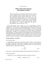
locations using a down-hole gamma logging technique. A posting of boring
locations is presented in Figure 7.1, with a schematic diagram of the site. At each
sampled location on the affected 20-acre portion of the site, a borehole was drilled
through the site surface soil, which contains the thorium bearing slag, typically to a
depth of about 15 feet. The boreholes were drilled with either 4- or 6-inch diameter
augers. Measurements in each borehole were performed starting from the surface
and proceeding downward in 6-inch increments.
The primary measurements were made with a 1x1 inch NaI detector (sodium
iodide) lowered into the borehole inside a PVC sleeve for protection. One-minute
gamma counts were collected (in the integral mode, no energy discrimination) at
each position using a “scaler.” Gamma counts were converted to thorium 232
(Th
232
) concentrations in pCi/gm using a calibration algorithm verified with
experimental data. The calibration algorithm includes background subtraction and
conversion of net gamma counts (counts per minute) to Th
232
concentration using a
semi-empirical detector response function and assumptions regarding the degree of
equilibrium between the gamma emitting thorium progeny and Th
232
in the soil.
The individual gamma logging measurements represent the “average”
concentration of Th
232
(or total thorium as the case may be) in a spherical volume
having a radius of approximately 12 to 18 inches. This volume “seen” by the down-
hole gamma detector is defined by the effective range in soil of the dominant gamma

ray energy (2.6 mev) emitted by thallium 208 (Tl
208
).
steqm-7.fm Page 164 Friday, August 8, 2003 8:19 AM
©2004 CRC Press LLC
Figure 7.1 Posting of Bore Hole Locations,
ABC Exotic Metals Site
steqm-7.fm Page 165 Friday, August 8, 2003 8:19 AM
©2004 CRC Press LLC
The Th
232
concentration measurements were subsequently converted to total
thorium to provide direct comparison to regulatory criteria expressed as
concentration of total thorium in soil. This assumed that Th
232
(the parent
radionuclide) and its decay series progeny are in secular equilibrium and thus total
thorium concentration (Th
232
plus Th
228
) is equal to two times the Th
232
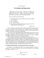
concentration. The histogram of the total thorium measurements is presented in
Figure 7.2. Note from this figure that more than 50 percent of the measurements are
reported as below the nominal method detection limit of 1 pCi/gm.
Geostatistical Modeling
Variograms
The processes distributing thorium containing slag around the ABCs site were
not random. Therefore, the heterogeneity of thorium concentrations at this site

cannot be expected to exhibit randomness, but, to exhibit spatial correlation. In
other words, total thorium measurement results taken “close together” are more
likely to be similar than results that are separated by “large” distances. There are
several ways to quantify the heterogeneity of measurement results as a function of
the distance between them (see Pitard, 1993; Isaaks and Srivastava, 1989). One of
the most useful is the “variogram,”
((h), which is half the average squared difference
between paired data values at distance separation h:
[7.1]
Figure 7.2 Frequency Diagram of Total Thorium Concentrations
γ h()
1
2N h()

t
i
t
j
–()
2
ij,()h
i
j
h=
∑
=
steqm-7.fm Page 166 Friday, August 8, 2003 8:19 AM
©2004 CRC Press LLC
Here N(h) is the number of pairs of results separated by distance h. The measured
total thorium data results are symbolized by t

1
, , t
n
.
Usually the value of the variogram is dependent upon the direction as well as
distance defining the separation between data locations. In other words, the
difference between measurements taken a fixed distance apart is often dependent
upon the directional axis considered. Therefore, given a set of data the values of γ (h)
maybe be different when calculated in the east-west direction than they are when
calculated in the north-south direction. This anisotropic behavior is accounted for by
considering “semi-variograms” along different directional axes. Looking at the
pattern generated by the semi-variograms often assists with the interpretation of the
spatial heterogeneity of the data. Further, if any apparent pattern of spatial
heterogeneity can be mathematically described as a function of distance and/or
direction, the description will assist in estimation of thorium concentrations at
locations where no measurements have been made.
Several models have been proposed to formalize the semi-variogram.
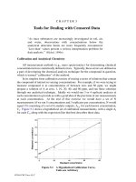
Experience has shown the spherical model has proven to be useful in many
situations. An ideal spherical semi-variogram is illustrated in Figure 7.3. The
formulation of the spherical model is as follows:
[7.2]
The spherical semi-variogram model indicates that observations very close
together will exhibit little variation in their total thorium concentration. This small
variation, referred to as the “nugget,” C
0
, represents sampling and analytical
variability, as well as any other source of “random” or unexplained variation. As
Figure 7.3 Ideal Spherical Model Semi-Variogram
Γ h() C
0

C
1
1.5
h
R

0.5
h
R



3
– hR<,+=
C
0
C
1
, h R≥+=
steqm-7.fm Page 167 Friday, August 8, 2003 8:19 AM
©2004 CRC Press LLC
illustrated in Figure 7.3, the variation between total thorium concentrations can be
expected to increase with distance separation until the total variation, C
0
+ C
1
, across
the site, or “sill,” is reached. The distance at which the variation reaches the sill is
referred to as the “range,” R. Beyond the range the measured concentrations are no
longer spatially correlated.

The practical significance of the range is that data points at a distance greater
than the range from a location at which an estimate is desired, provide no useful
information regarding the concentration at the desired location. This very important
consideration is largely ignored by many popular interpolation algorithms including
inverse distance weighting.
Estimation via Ordinary “Kriging”
The important task of estimation of the semi-variogram models is also often
overlooked by those who claim to have applied geostatistical analysis by using
“kriging” to estimate the extent of soil contamination. The process of “kriging” is
really the second step in geostatistical analysis, which seeks to derive an estimate of
concentration at locations where no measurement has been made. The desired
estimator of the unknown concentration, t
A
, should be a linear estimate from the
existing data, t
1
, , t
n
. This estimator should be unbiased in that on the average, or
in statistical expectation, it should equal the “true” concentration at that point. And,
the estimator should be that member of the class of “linear-unbiased” estimators that
has minimum variance (is the “best”) about its true value. In other words, the desired
kriging estimator is the “best linear unbiased” estimator of the true unknown value,
T
A
. These are precisely the conditions that are associated with ordinary linear least
squares estimation.
Like the derivation of ordinary linear least squares estimators, one begins with
the following relationship:
[7.3]

That is, the estimate of unknown concentration at a geographical location, t
A
, is a
weighted sum of the observed concentrations, the t’s, in the same “geostatistical
neighborhood” of the location for which the estimate is desired.
Calculating and minimizing the error variance in the usual way one obtains the
following “normal” equations:

[7.4]

w
1
+ w
2
+ … + w
n
= 1
t
A
w
1
t
1
w
2
t
2
w
3
t

3
… w
n
t
n
++++=
w
1
V
11,
w
2
V
12,
… w
n
V
1n,
LV
1A,
=++++
w
1
V
21,
w
2
V
22,
… w

n
V
2n,
LV
2A,
=++++
w
1
V
n1,
w
2
V
n2,
… w
n
V
nn,
LV
nA,
=++++
steqm-7.fm Page 168 Friday, August 8, 2003 8:19 AM
©2004 CRC Press LLC
Here V
i,j
is the covariance between t
i
and t
j
and, L is the mean of a random

function associated with a particular location symbolized by . The symbol will
be used to designate the three-dimensional location vector (x, y, z).
Geostatistics deal with random functions, in addition to random variables. A
random function is a set of random variables {t | location belongs to the area of
interest} where the dependence among these variables on each other is specified by
some probabilistic mechanism. The random function expresses both the random and
structured aspects of the phenomenon under study as:
• Locally, the point value is considered a random variable.
• The point value is also a random function in the sense that for each pair
of points and , the corresponding random variables and
are not independent but related by a correlation expressing the
spatial structure of the phenomenon.
In addition, linear geostatistics consider only the first two moments, the mean and
variance, of the spatial distribution of results at any point . It is therefore assumed
that these moments exist and exhibit second-order stationarity. The latter means that
(1) the mathematical expectation, , exists and does not depend on location ;
and, (2) for each pair of random variables, , the covariance exists
and depends only on the separation vector .
In this context, the covariances, V
i,j
’s, in the above system of linear equations
can be replaced with values of the semi-variograms. This leads to the following
system of linear equations for each particular location:
w
1
'
1,1
+ w
2
'

1,2
+ + w
n
'
1,n
+ L = '
1,A
w
1
'
2,1
+ w
2
'
2,2
+ + w
n
'
2,n
+ L = '
2,A

[7.5]

w
1
'
n,1
+ w
2

'
n,2
+ + w
n
'
n,n
+ L = '
n,A
w
1
+ w
2
+ + w
n
= 1
Solving this system of equations for the w’s yields the weights to apply to the
measured realizations of the random variables, the t’s, to provide the desired
estimate.
Discussion of the basic concepts and tools of geostatistical analysis can be
found in the excellent books by Goovaerts (1997), Isaaks and Srivastava (1989), and
Pannatier (1996). These techniques are also discussed in Chapter 10 of the U. S.
Environmental Protection Agency (USEPA) publication, Statistical Methods for
Evaluating the Attainment of Cleanup Standards. Volume 1: Soils and Solid Media
(1989).
Journel (1988) describes the advantages and disadvantages of ordinary kriging
as follows:
x
x
x() x
tx()

tx()
x
i
x
i
h+ tx
i
()
tx
i
h+()
x
Etx(){} x
tx
i
() tx
i
h+(),{}
h
steqm-7.fm Page 169 Friday, August 8, 2003 8:19 AM
©2004 CRC Press LLC
“Traditional interpolation techniques, including triangularization
and inverse distance weighting, do not provide any measure of
the reliability of the estimates The main advantage of
geostatistical interpolation techniques, essentially ordinary
kriging, is that an estimation variance is attached to each
estimate Unfortunately, unless a Gaussian distribution of
spatial errors is called for, an estimation variance falls short of
providing confidence intervals and the error probability
distribution required for risk assessment.

Regarding the characterization of uncertainty, most interpolation
algorithms, including kriging, are parametric; in the sense that a
model for the distribution of errors is assumed, and parameters of
that model (such as the variance) are provided by the algorithm.
Most often that model is assumed normal or at least symmetric.
Such congenial models are perfectly reasonable to characterize
the distribution of, say, measurement errors in the highly
controlled environment of a laboratory. However they are
questionable when used for spatial interpolation errors ”
In addition to doubtful distributional assumptions, other problems associated
with the use of ordinary kriging at sites such as the ABC Metals site are:
• How are measurements recorded as below background to be handled in
statistical calculations? Should they assume a value of one-half background,
or a value equal to background, or assumed to be zero? (See Chapter 5,
Censored Data.)
• There are several cases where the total thorium concentrations vary greatly
with very small changes in depth, as well as evidence that the variation in
measured concentration is occasionally quite large within small areal
distances. A series of borings in an obvious area of higher concentration at
the ABC Metals site exhibit large differences in concentration within an areal
distance as small as four feet. How these cases are handled in estimating the
semi-variogram model will have a critical effect on derivation of the
estimation weights.
Decisions made regarding the handling of measurements less than background
may bias the summary statistics including the sample semi-variograms. The
techniques suggested for statistically dealing with such observations are often
cumbersome to apply (USEPA, 1996) and if such data are abundant may only be
effectively dealt with via nonparametric statistical methods (U.S. Nuclear
Regulatory Commission, 1995). The effect of the latter condition on estimation of
the semi-variogram model is that the “nugget” is apparently equivalent to the sill.

This being the case, the concentration variation at the site would appear to be random
and any spatial structure related to the “occurrence” of high values of concentration
steqm-7.fm Page 170 Friday, August 8, 2003 8:19 AM
©2004 CRC Press LLC
will be masked. If the level of concentration at the site is truly distributed at random,
as implied by a semi-variogram with the nugget equal to the sill and a range of zero,
then the concentration observed at one location tells us absolutely nothing about the
concentration at any other location. An adequate estimate of concentration at any
desired location may be simply made in such an instance by choosing a
concentration at random from the set of observed concentrations.
Measured total thorium concentrations in the contaminated areas of the site span
orders of magnitude. Because the occurrence of high measured total thorium
concentration is relatively infrequent, the technique developed by André Journel
(1983a, 1983b, 1988) and known as “Probability Kriging” offers a solution to
drawbacks of ordinary kriging.
Nonparametric Geostatistical Analysis
Journel (1988) suggests that instead of estimating concentration directly,
estimate the probability distribution of concentration measurements at each location.
“ Non-parametric geostatistical techniques put as a priority,
not the derivation of an “optimal” estimator, but modeling of the
uncertainty. Indeed, the uncertainty model is independent of the
particular estimate retained, and depends only on the
information (data) available. The uncertainty model takes the
form of a probability distribution of the unknown rather than
that of the error, and is given in the non-parametric format of a
series of quantiles.”
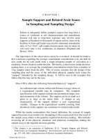
The estimation of the desired probability distribution is facilitated by first
considering the empirical cumulative distribution function (ecdf) of total thorium
concentration at the site. The ecdf for the observations made at the ABC site is given
in Figure 7.4. It is simply constructed by ordering the total thorium concentration

observations and plotting the relative frequency of occurrence of concentrations less
than the observed measurement. The concept of the ecdf and its virtues was
introduced and discussed in Chapter 6.
Note that by using values of the ecdf instead of the thorium concentrations
directly, at least two of the major issues associated with ordinary kriging are
resolved. The relatively large changes in concentration due to a few high values
translate into small changes in the relative frequency that these total thorium
concentration observations are not exceeded. If the relative frequency that a
concentration level is not exceeded is the subject of geostatistical analysis, instead of
the observations themselves, the effect on estimating semi-variogram models of
large changes in concentration over small distances is diminished. Thus the
resulting estimated semi-variograms are very resistant to outlier data.
Further, issues regarding which value to use for measurements reported as less
than background in statistical calculations become moot. All such values are assigned
the maximum relative frequency associated with their occurrence. The maximum
relative frequency is appropriate because it is the value of a right-continuous ecdf. In
steqm-7.fm Page 171 Friday, August 8, 2003 8:19 AM
©2004 CRC Press LLC
other words, it is desired to describe the cumulative histogram of the data with a
continuous curve. To do so it is appropriate to draw such a curve through the upper
right-hand corner of each histogram bar.
The desired estimator of the probability distribution of total thorium
concentration at any point, , is obtained by modeling probabilities for a series of K
concentration threshold values T
k
discretizing the total range of variation in
concentration. This is accomplished by taking advantage of the fact that the
conditional probability of a measured concentration, t, being less than threshold T
k
is the conditional expectation of an “indicator” random variable, I

k
. I
k
is defined as
having a value of one if t is less than threshold T
k
, and a value of zero otherwise.
Four threshold concentrations have been chosen for this site. These are 3, 20,
45, and 145 pCi/gm as illustrated in Figure 7.4. The rationale for choosing precisely
these four thresholds is that the ecdf between these thresholds, and between the
largest threshold and the maximum measured concentration may be reasonably
represented by a series of linear segments. The reason as to why this is desirable will
become apparent later in this chapter.
The data are now recoded into four new binary variables, (I
1
, I
2
, I
3
, I
4
)
corresponding to the four thresholds as indicated above. This is formalized as
follows:
[7.6]
It is possible to obtain kriged estimators for each of the indicators . The
results of such estimation will yield conditional probabilities of not exceeding each
Figure 7.4 Empirical Cumulative Distribution Function Total Thorium
x
I

k
x() 1if tx() T
k
≤ 0 if t x() T
k
>,;,=
I
k
x()
steqm-7.fm Page 172 Friday, August 8, 2003 8:19 AM
©2004 CRC Press LLC
of the four threshold concentrations at point . These estimates are of the local
indicator mean at each location. These estimates are exact in that they reproduce the
observed indicator values at the datum locations. However, estimates of the
probability of exceeding the indicator threshold are likely to be underestimated in
areas of lower concentration and overestimated in areas of higher concentration
(Goovaerts, 1997, pp. 293–297). Obtaining “kriged” estimates of the indicators
individually ignores indicator data at other thresholds different from that being
estimated and therefore does not make full use of the available information.
The additional information provided by the indicators for the “secondary”
thresholds can be taken into account by using “cokriging,” which explicitly accounts
for the spatial cross-correlation between the primary and secondary indicator
variables (see Goovaerts, 1997, pp. 185–258). The unfortunate part of indicator
cokriging with K indicator variables is that one must infer and jointly estimate K
direct and K(K − 1)/2 cross semi-variograms. If anisotropy is present, meaning that
the semi-variogram is directionally dependent, this may have to be done in each of
three dimensions. In our present example this translates into 10 direct and cross
semi-variograms in each of three dimensions.
Once we have accomplished this feat we then may obtain estimates of the
probability that an indicator threshold is, or is not, exceeded that will have

theoretically smaller variance than that obtained by using the individual threshold
indicators. Goovaerts (1997, pp. 297–300) discusses the virtues and problems
associated with indicator cokriging. One of the drawbacks is that when we are
finished we only have estimates of the probability that the threshold concentration is,
or is not, exceeded at those concentration thresholds chosen. We may refine our
estimation by choosing more threshold concentrations and defining more indicators.
Thus we may obtain a better definition of the conditional cumulative distribution at
the expense of more direct and cross semi-variograms to infer and estimate. This can
rapidly become a daunting task.
To make the process manageable, cokriging of the indicator transformed data
using the rank-order transform of the ecdf, symbolized by U, as a secondary variable
offers a solution. This process is referred to as probability kriging (PK). Goovaerts
(1997), Isaaks (1984), Deutsch and Journel (1992), and Journel (1983a, 1983b,
1988) present nice discussions of the nonparametric geostatistical analysis process
sometimes referred to as “probability kriging.” Other advantages in terms of
interpreting the results are discussed by Flatman et al. (1985).
The appropriate PK estimator at point A given the local information in the
neighborhood of A is:
[7.7]
The weights
8
m
, <
m
are obtained as the solution to the following system of
linear equations:
x
I
Ak
Σ

m1n,=
λ
m
I
mk
Σ
m1n,=
ν
m
U
m
+ Prob t
A
T
k
≤[]==
steqm-7.fm Page 173 Friday, August 8, 2003 8:19 AM
©2004 CRC Press LLC
[7.8]
The above system of equations demands that semi-variograms be established
for each of the indicators I
k
’s, the rank-order transform of the ecdf U, and the
covariance between each of the I
k
’s and U. The sample values of the required semi-
variograms are obtained as the following:
[7.9]
Indicator Semi-Variogram
[7.10]

Uniform Transform Semi-Variogram
[7.11]
Cross Semi-Variogram
The cross semi-variogram describes the covariance between the indicator
variable and the uniform transform variable.
The values of the sample semi-variograms and cross-variograms can be used to
estimate the parameters of their corresponding spherical models. These models are
as follows for the kth indicator variable:
[7.12]
λ
ik,
Γ
I
k
,(i,j)
ν
i,k
Γ
IU
k
,(i,j)
L
I
i
+
i=1
n
∑
+
i=1

n
∑
Γ
I
A
,(i,A)
, j = 1, , n=
λ
ik,
Γ
IU
k
,(i,j)
ν
i,k
Γ
U
k
,(i,j)
L
U
i
+
i=1
n
∑
+
i=1
n
∑

Γ
IU
A
,(i,A)
, j = 1, , n=
λ
ik,
i=1
n
∑
1=
ν
ik,
i=1
n
∑
0=
γ
I
k
h()
1
2N h()

I
ki,
I
kj,
–()
2

ij,()h
i
j
h=
∑
=
γ
U
h()
1
2N h()

U
i
U
j
–()
2
ij,()h
i
j
h=
∑
=
γ
IU
k
h()
1
2N h()

I
ki,
I
kj,
–()U
i
U
j
–()
ij,()h
i
j
h=
∑
=
Γ
k
h() C
I
k
,0
C
I
k
,1
1.5
h
R
1

0.5
h
R
1



3
– C
I
k
,2
1.5
h
R
2

0.5
h
R
2



3
– h < R
1
< R
2

,++=
C
I
k
,0
C
I
k
,1
C
I
k
,2
1.5
h
R
2

0.5
h
R
2



3
– R
1
< h < R
2

,++=
C
I
k
,0
C
I
k
,1
C
I
k
,2
R
1
< R
2
< h,++=
steqm-7.fm Page 174 Friday, August 8, 2003 8:19 AM
©2004 CRC Press LLC
The model for the uniform transformation variable is:
[7.13]
For the cross-variograms the models are defined as:
[7.14]
Note that these models contain two ranges, R
1
and R
2
, and associated sill
coefficients, C

1
and C
2
, reflecting the presence of two plateaus suggested by the
sample semi-variograms. This representation defines a “nested” structural model for
the semi-variogram. The sample and estimated models for semi-variograms are
presented in the Figures 7.5–7.8. The estimated semi-variogram model is
represented by the continuous curve, and the sample semi-variogram is represented
by the points shown in these figures.
There are 27 semi-variograms appearing in Figures 7.5–7.8. Because of the
geometric anisotropy indicated by the data, nine variograms are required in each of
three directions. These nine semi-variograms are distributed as one for the uniform
transformed data, four for the indicator variables and four cross semi-variograms
between the uniform transform and each of the indicator variables.
The derivation of the semi-variogram models employed the software of GSLIB
(Deutsch and Journel, 1992) to calculate the sample semi-variograms and SAS/Stat
(SAS, 1989) software to estimate the ranges and structural coefficients of the semi-
variogram models. Estimation of the structural coefficients, i.e., the nugget and sills,
involves nonlinear estimation procedures constrained by the requirements of
coregionalization. This simply means that the semi-variogram structures for an
indicator variable, that for the uniform transform and their cross semi-variogram
must be consonant with each other. Coregionalization demands that coefficients
C
I,m
and C
U,m
be greater than zero, for all m = 0, 1, 2, and that the following
determinant be positive definite:
C
I,m

C
UI,m
[7.15]
C
UI,m
C
U,m
Γ
U
h() C
U,0
C
U,1
1.5
h
R
1

0.5
h
R
1



3
– C
U,2
1.5
h

R
2

0.5
h
R
2



3
– ,h <R
1
<R
2
++=
C
U,0
C
U,1
C
U,2
1.5
h
R
2

0.5
h
R

2



3
– , R
1
< h < R
2
++=
C
U,0
C
U,1
C
U,2
, R
1
< R
2
< h++=
Γ
UI
k
h() C
UI
k
,0
+ C
UI

k
,1
1.5
h
R
1

0.5
h
R
1



3
– + C
UI
k
,2
1.5
h
R
2

0.5
h
R
2




3
– ,=
h < R
1
< R
2
C
UI
k
,0
+ C
UI
k
,1
+ C
UI
k
,2
1.5
h
R
2

0.5
h
R
2




3
– R
1
< h < R
2
,=
C
UI
k
,0
+ C
UI
k
,1
+ C
UI
k
,2
, R
1
< R
2
< h=
steqm-7.fm Page 175 Friday, August 8, 2003 8:19 AM
©2004 CRC Press LLC
Figure 7.5A N-S Indicator Semi-variograms
Semi-variogram
steqm-7.fm Page 176 Friday, August 8, 2003 8:19 AM
©2004 CRC Press LLC

Figure 7.5B N-S Indicator Semi-variograms
Cross Semi-variogram
steqm-7.fm Page 177 Friday, August 8, 2003 8:19 AM
©2004 CRC Press LLC
Figure 7.6A E-W Indicator Semi-variograms
Semi-variogram
steqm-7.fm Page 178 Friday, August 8, 2003 8:19 AM
©2004 CRC Press LLC
Figure 7.6B E-W Indicator Semi-variograms
Cross Semi-variogram
steqm-7.fm Page 179 Friday, August 8, 2003 8:19 AM
©2004 CRC Press LLC
Figure 7.7A Vertical Indicator Semi-variograms
Semi-variogram
steqm-7.fm Page 180 Friday, August 8, 2003 8:19 AM
©2004 CRC Press LLC
Figure 7.7B Vertical Indicator Semi-variograms
Cross Semi-variogram
steqm-7.fm Page 181 Friday, August 8, 2003 8:19 AM
©2004 CRC Press LLC
Figure 7.8 Uniform Transform Semi-variograms
steqm-7.fm Page 182 Friday, August 8, 2003 8:19 AM
©2004 CRC Press LLC
The coregionalization requirements lead to the following practical rules:
• Any structure that appears in the cross semi-variogram must also appear in
both the indicator and uniform semi-variograms.
• A structure appearing in either the indicator or uniform semi-variograms does
not necessarily have to appear in the cross semi-variogram model.
While one might argue that some of the semi-variogram models do not appear to fit
the sample semi-variograms very well, in practice an assessment must be made as to

whether improving the fit of all semi-variograms is worth the effort. If by doing so
has little effect on estimation and significantly complicates specification of the
kriging model it probably is not worth the additional effort. Such was the judgment
made here.
Some Implications of Variography
The semi-variograms provide some interesting information regarding the spatial
distribution of total thorium at the site. The semi-variogram models for the first three
indicators and the uniform transform are described by variogram models (see Figures
7.5–7.8) with an isotropic nugget effect and two additional transition structures as
described above. The first of the transition structures exhibits a range of 50 feet and
is isotropic in the horizontal (x, y) plane but shows directional anisotropy between
the vertical (z) and the x, y plane. The second transition structure exhibits directional
anisotropy among all directions. Directional anisotropy is characterized by constant
sill coefficients, C
1
and C
2
, and directionally dependent ranges for each transition
structure.
The directional anisotropy in the x, y plane is interesting. The estimated range
along the north-south axis is 1,000 feet, but only 750 feet in the east-west direction.
This suggests that where low to moderate thorium concentrations are found, they
will tend to occur in elliptical regions with the long axis oriented in a north-south
direction. This orientation is consonant with the facility layout and traffic patterns.
The semi-variogram models for the 145 pCi/gm indicator appear to be isotropic
in the x, y plane and exhibit only one transition structure. The range of this transition
structure is estimated to be 50 feet. This suggests that when high concentrations of
total thorium are found, they tend to define rather confined areas. Note that this
indicator exhibits one transition structure in the vertical direction. This suggests that
the horizontally confined areas of high concentration tend to be confined in the

vertical direction as well.
There are tools other than the semi-variogram for investigating the relationship
among observations as a function of their distance separation. These include the
“Standardized Variogram,” the “Correlogram,” and the “Madogram.” These are
mentioned here without definition to recognize their existence. Their definition is
not necessary to our discussion as to why one needs to pay attention to the structure
of the spatial relationships among observations. The interested reader is referred to
Goovaerts (1997), Isaaks and Srivastava (1989), and Pannatier (1996), among
others, for a complete discussion of these tools.
steqm-7.fm Page 183 Friday, August 8, 2003 8:19 AM
©2004 CRC Press LLC
In addition to providing insight into the deposition process and possible changes
in the deposition process that might occur for different concentration ranges,
variography also permits an assessment of sampling adequacy. It was mentioned
earlier that observations at a distance away from a point of interest that is greater
than the range provide no information about the point of interest. Thus the ranges
associated with the directional semi-variograms define an ellipsoidal
“neighborhood” about a point of interest in which we may obtain information about
the point of interest. A practical rule-of-thumb is that this neighborhood is defined
by axes equivalent to two-thirds the respective range.
Looking at the collection of available samples, should we find that there are no
samples within the neighborhood of a point of interest, then the existing collection of
samples is inadequate. We have also indicated the physical locations for the
collection of additional samples. The interpolation algorithms often found with
Geographical Information System (GIS), including the popular inverse-weighted
distance algorithm, totally ignore the potential inadequate sampling problem.
Estimated Distribution of Total Thorium Concentration
Once the semi-variogram models were obtained they were used to estimate the
conditional probability distribution of total thorium concentration at the centroid of
253,344 blocks across the site. Kriged estimates were obtained for each block of

dimension 2.5 m by 2.5 m by 0.333m (8.202 ft by 8.202 ft by 1.094 ft) to a nominal
depth of 15 feet. The depth restriction is imposed because only a very few borings
extend to, or beyond, that depth. All measured concentrations beyond a depth of
15.5 feet are recorded as below background. Each block is oriented according to the
usual coordinate axes.
Truly three-dimensional PK estimation was performed to obtain the conditional
probability that the total thorium concentration will not exceed each of the four
indicator concentrations. This estimation employed PK software developed
specifically for Splitstone & Associates by Clayton Deutsch, Ph.D., P.E. (1998) while
at Stanford University. PK estimation was restricted to use up to 8 nearest data values
within an elliptical search volume centered on the point of estimation. The principal
axes of this elliptical region were chosen as 670 ft, 500 ft, and 10 ft in the principal
directions. The lengths of these axes correspond to approximately two-thirds of the
effective directional ranges. During semi-variogram estimation it was concluded that
no rotation of the principal axes from their usual directions was necessary.
Upon completion of PK, the grid network of points of estimation was restricted
to account for the irregular site boundary and other salient features such as buildings
and roads existing prior to the production of the ferrocolumbium alloy. It makes
logical sense to impose this restriction on the mathematical estimation as the thorium
slag is not mobile. Figure 7.9 shows the areal extent of block grid after applying
restrictions. This grid defines the areal centroid locations of 152,124 “basic remedial
blocks” of volume 2.7258 cubic yards (cu yds).
The results immediately available upon completion of PK estimation are the
conditional probabilities that the total thorium concentration will not exceed each of
the four indicator concentrations at each point of estimation. Because the basic
steqm-7.fm Page 184 Friday, August 8, 2003 8:19 AM
©2004 CRC Press LLC
Figure 7.9 PK Estimation Grid Schematic
steqm-7.fm Page 185 Friday, August 8, 2003 8:19 AM
©2004 CRC Press LLC

blocks size is “small” relative to the majority of data spacing, these probabilities may
be considered as defining the relative frequency of occurrence of all possible
measurements made within the block.
While it certainly is beneficial to know the conditional probabilities that the
total thorium concentration will not exceed each of the four indicator concentrations,
other statistics may be more useful for planning decommissioning activities. For
instance, it is useful to know what concentration levels will not be exceeded with a
given probability. These concentrations, or quantiles, can be easily obtained by
using the desired probability and the PK results to interpolate the ecdf. This is why
an approximate linear segmentation of the ecdf when choosing the indication
concentrations is of value. Twenty-two quantile concentrations were estimated for
each block corresponding to the following percentiles of the distribution: the 5th,
10th, 20th, 30th, 40th, 45th, 50th, 55th, 60th, 63th, 65th, 67th, 70th, 73th, 75th, 77th,
80th, 82nd, 85th, 87th, 90th, and 95th.
In addition to the various quantile estimates of total thorium concentration, the
expected value, or mean, total thorium concentration for any block may be obtained.
The expected value is easily calculated as the weighted average of the mean ecdf
concentrations found between the indicator concentration values, or an indicator
concentration and the minimum or maximum observed concentration as appropriate.
The weights are supplied by the incremental PK estimated probabilities.
Other statistics of potential interest in planning for decommissioning may be the
probabilities that certain fixed concentrations are exceeded (or not exceeded). These
fixed concentrations are defined by the NRC dose criteria for release for unrestricted
use and restricted-use alternatives:
• greater than 10 pCi/gm
• greater than 25 pCi/gm, and
• greater than 130 pCi/gm.
Conditional estimates of the desired probabilities can be easily obtained by using the
desired concentrations and the PK results to interpolate the ecdf.
All of these estimates are labeled “conditional.” However, it is important to

realize that they are conditional only on the measured concentration data available.
This condition is one that applies to any estimation method. If the data change, then
the estimates may also change. Nonparametric geostatistics require no other
assumptions, unlike other estimation techniques.
Figures 7.10 through 7.14 present a depiction of estimated conditional
concentration densities for “typical” basic blocks that fall into different concentration
ranges. Note that the shape of the distribution will change from block to block. The
concentration scale of these figures is either logarithmic or linear to enhance the
visualization of the densities.
Figure 7.10 illustrates the conditional density of total thorium concentration for
a location having a better than 80 percent chance of meeting the unrestricted release
criterion. It is important to realize that even with this block there is a finite, albeit
very small, probability of obtaining a measurement result for total thorium
exceeding 130 pCi/gm.
steqm-7.fm Page 186 Friday, August 8, 2003 8:19 AM
©2004 CRC Press LLC

Figure 7.11 illustrates the conditional density for a “typical” block, which may
be classified in concentration range between 10 and 25 pCi/gm. Note that for this
block there is a better than 60 percent chance of a measured concentration being
below 25 pCi/gm.
Figure 7.10 “Typical” Density Block Type 1
Figure 7.11 “Typical Density Block Type 2
steqm-7.fm Page 187 Friday, August 8, 2003 8:19 AM
©2004 CRC Press LLC