Statistical Tools for Environmental Quality Measurement - Chapter 8 (end) ppt

C H A P T E R 8
Tools for the Analysis of Temporal Data
“In applying statistical theory, the main consideration is not what
the shape of the universe is, but whether there is any universe at
all. No universe can be assumed, nor statistical theory
applied unless the observations show statistical control.”
“ Very often the experimenter, instead of rushing in to apply
[statistical methods] should be more concerned about attaining
statistical control and asking himself whether any predictions at
all (the only purpose of his experiment), by statistical theory or
otherwise, can be made.” (Deming, 1950)
All too often in the rush to summarize available data to derive indices of
environmental quality or estimates of exposure, the assumption is made that
observations arise as a result of some random process. Actually, experience has
shown that the statistical independence of environmental measurements at a point of
observation is a rarity. Therefore, the application of statistical theory to these
observations, and resulting inferences are simply not correct.
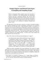
Consider the following representation of hourly concentrations of airborne
particulate matter less than 10 microns in size (PM
10
) made at the Liberty Borough
monitoring site in Allegheny County, Pennsylvania, from January 1 through
August 31, 1993.
Figure 8.1 Hourly PM
10
Observations,
Liberty Borough Monitor, January–August 1993
Fine Particulate(PM10), ug/Cubic
0 40 80 120 160 200 240 280 320 360
Relative Frequency
Fine Particulate (PM10), ug/Cubic

steqm-8.fm Page 203 Friday, August 8, 2003 8:21 AM
©2004 CRC Press LLC
The shape of this frequency diagram of PM
10
concentration is typical in air
quality studies, and popular wisdom frequently suggests that these data might be
described by the statistically tractable log-normal distribution. However, take a look
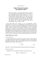
at this same data plotted versus time.
Careful observation of this figure suggests that the concentrations of PM
10
tend
to exhibit an average increase beginning in May. Further, there appears to be a short-
term cyclic behavior on top of this general increase. This certainly is not what would
be expected from a series of measurements that are statistically independent in time.
The suggestion is that the PM
10
measurements arise as a result of a process having
some definable “structure” in time and can be described as a “time series.”
Other examples of environmental time series are found in the observation of
waste water discharges; groundwater analyte concentrations from a single well,
particularly in the area of a working landfill; surface water analyte measurements
made at a fixed point in a water body; and, analyte measurements resulting from the
frequent monitoring of exhaust stack effluent. Regulators, environmental
professionals, and statisticians alike have traditionally been all too willing to assume
that such series of observations arise as statistical, or random, series when in fact
they are time series. Such an assumption has led to many incorrect process
compliance performances, and human exposure decisions.
Our decision-making capability is greatly improved if we can separate the
underlying “signal,” or structural component of the time series, from the “noise,” or
“stochastic” component. We need to define some tools to help us separate the signal

from the noise. Like the case of spatially related observations, useful tools will help
us to investigate the variation among observations as a function of their separation
Figure 8.2 Hourly PM
10
Observations versus Time,
Liberty Borough Monitor, January–August, 1993
PM10, ug/Cubic Meter
01JAN93 01MAR93 01MAY93 01JUL93 01SEP93
1
10
100
1000
steqm-8.fm Page 204 Friday, August 8, 2003 8:21 AM
©2004 CRC Press LLC
distance, or “lag.” Unlike spatially related observations, the temporal spacing of
observations has only one dimension, time.
Basis for Tool Development
It seems reasonable that the statistical tools used for investigating a temporal
series of observations ordered in time, (z
1
, z
2
, z
3
, z
N
), should be based upon
estimation of the variance of these observations as a function of their spacing in time.
Such a tool is provided by the sample “autocovariance” function:
k = 0, 1, 2, , K [8.1]

Here, represents the mean of the series of N observations.
If we imagine that the time series represents a series of observations along a
single dimension axis in space, then the astute reader will see a link between the
covariance described by [8.1] and the variogram described by Equation [7.1]. This
link is as follows:
[8.2]
The distance, k, represents the k
th
unit of time spacing, or lag, between time series
observations.
A statistical series that evolves in time according to the laws of probability is
referred to as a “stochastic” series or “process.” If the true mean and autocovariance
are unaffected by the time origin, then the stochastic process is considered to be
“stationary.” A stationary stochastic process arising from a Normal, or Gaussian,
process is completely described by its mean and covariance function. The
characteristic behavior of a series arising from Normal measurement “error” is a
constant mean, usually assumed to be zero, and a constant variance with a
covariance of zero among successive observations for greater than zero lag, (k > 0).
Deviations from this characteristic pattern suggest that the series of observations
may arise from a process with a structural as well as a stochastic component.
Because it is the “pattern” of the autocovariance structure, not the magnitude,
that is important, it is convenient to consider a simple dimensionless transformation
of the autocovariance function, the autocorrelation function. The value of the
autocorrelation, r
k
, is simply found by dividing the autocovariance [8.1] by the
variance, C
0
:
[8.3]

The sample autocorrelation function of the logarithm of PM
10
concentrations
presented in Figure 8.2 is shown below for the first 72 hourly lags. This figure
C
k
1
N

z
t
z–()z
tk+
z–(),
t1=
NK–
∑
=
z
γ k() C
0
C
k
–=
r
k
C
k
C
0

k
, 012… K,,,,==
steqm-8.fm Page 205 Friday, August 8, 2003 8:21 AM
©2004 CRC Press LLC
illustrates a pattern that is much different from that characteristic of measurement
error. It certainly indicates that observations separated by only one hour are highly
related (correlated) to one another. The correlation, describing the strength of
similarity in time among the observations, decreases as the distance separation, the
lag, increases.
A number of estimates have been proposed for the autocorrelation function.
The properties are summarized in Jenkins and Watts (2000). It is concluded that the
most satisfactory estimate of the true kth lag autocorrelation is provided by [8.3].
It is necessary to discuss some of the more theoretical concepts regarding
“general linear stochastic models” to assist the reader in appreciation of the
techniques we have chosen for investigating and describing time series data. Few, if
any, of the time series found in environmental studies result from stationary
processes that remain in equilibrium with a constant mean. Therefore, a wider class
of nonstationary processes called autoregressive-integrated moving average
processes (ARIMA processes) must be considered. This discussion is not intended
to be complete, but only to provide a background for the reader.
Those interested in pursuing the subject are encouraged to consult the classic
work by Box et al. (1994), Time Series Analysis Forecasting and Control.
Somewhat more accessible accounts of time series methodology can be found in
Chatfield (1989) and Diggle (1990). An effort has been made to structure the
following discussion of theory, nomenclature, and notation to follow that used by
Box and Jenkins.
Figure 8.3 Autocorrelation of Ln Hourly PM
10
Observations,

Liberty Borough Monitor, January–August 1993
Autocorrelation
0.0
0.2
0.4
0.6
1.0
0.8
Lag. Hours
0 6 12 18 24 30 36 42 48 54 60 66 72
steqm-8.fm Page 206 Friday, August 8, 2003 8:21 AM
©2004 CRC Press LLC
It should be mentioned at this point that the analysis and description of time
series data using ARIMA process models is not the only technique for analyzing
such data. Another approach is to assume that the time series is made up of sine and
cosine waves with different frequencies. To facilitate this “spectral” analysis, a
Fourier cosine transform is performed on the estimate of the autocovariance
function. The result is referred to as the sample spectrum. The interested reader
should consult the excellent book, Spectral Analysis and Its Applications, by Jenkins
and Watts (2000).
Parenthetically, this author has occasionally found that spectral analysis is a
valuable adjunct to the analysis of environmental times series using linear ARIMA
models. However, spectral models have proven to be not nearly as parsimonious as
parametric models in explaining observed variation. This may be due in part to the
fact that sampling of the underlying process has not taken place at precisely the
correct frequency in forming the realization of the time series. The ARIMA models
appear to be less sensitive to the “digitization” problem.
ARIMA Models — An Introduction
ARIMA models describe an observation made at time t, say z
t

, as a weighted
average of previous observations, z
t− 1
, z
t− 2
, z
t− 3
, z
t− 4
, z
t− 5
, , plus the weighted
average of independent, random “shocks,” a
t
, a
t− 1
, a
t− 2
, a
t− 3
, a
t− 4
, a
t− 5
, This
leads to the expression of the current observation, z
t
, as the following linear model:
z
t

= φ
0
+ φ
1
z
t− 1
+ φ
2
z
t− 2
+ φ
3
z
t− 3
+ + a
t
- θ
1
a
t− 1
− θ
1
a
t− 2
− θ
1
a
t− 3
−
The problem is to decide how many weighting coefficients, the φ ’s and θ ’s, should

be included in the model to adequately describe z
t
and secondly, what are the best
estimates of the retained φ ’s and θ ’s. To efficiently discuss the solution to this
problem, we need to define some notation.
A simple operator, the backward shift operator B, is extensively used in the
specification of ARIMA models. This operator is defined by Bz
t
= z
t− 1
; hence,
B
m
z
t
= z
t− m
. The inverse operation is performed by the forward shift operator F = B
− 1
given by Fz
t
= z
t+1
; hence, F
m
z
t
= z
t+m
. The backward difference operator, ∇ , is

another important operator that can be written in terms of B, since
The inverse of ∇ is the infinite sum of the binomial series in powers of B:
∇ z
t
z
t
z
t-1
– 1B–()z
t
==
∇
1–
z
t
z
t-j
j=0
∞
∑
z
t
z
t-1
z
t-2
…+++==
1BB
2
…++ +()z

t
=
1B–()
1–
z
t
=
steqm-8.fm Page 207 Friday, August 8, 2003 8:21 AM
©2004 CRC Press LLC
Yule (1927) put forth the idea that a time series in which successive values are
highly dependent can be usefully regarded as generated from a series of independent
“shocks,” a
t
. The case of the damped harmonic oscillator activated by a force at a
random time provides an example from elementary physical mechanics. Usually,
the shocks are thought to be random drawings from a fixed distribution assumed to
be normal with zero mean and constant variance . Such a sequence of random
variables a
t
, a
t− 1
, a
t− 2
, is called white noise by process engineers.
A white noise process can be transformed to a nonwhite noise process via a
linear filter. The linear filtering operation simply is a weighted sum of the previous
realizations of the white noise a
t
, so that
[8.4]

The parameter µ describes the “level” of the process, and
[8.5]
is the linear operator that transforms a
t
into z
t
. This linear operator is called the
transfer function of the filter. This relationship is shown schematically.
The sequence of weights ψ
1
, ψ
2
, ψ
3
, may, theoretically, be finite or infinite.
If this sequence is finite, or infinite and convergent, then the filter is said to be stable
and the process z
t
to be stationary. The mean about which the process varies is given
by µ. The process z
t
is otherwise nonstationary and µ serves only as a reference
point for the level of the process at an instant in time.
Autoregressive Models
It is often useful to describe the current value of the process as a finite weighted
sum of previous values of the process and a shock, a
t
. The values of a process z
t
, z

t-1
,
z
t− 2
, , taken at equally spaced times t, t − 1, t − 2, , may be expressed as
deviations from the series mean forming the series ; where
. Then
[8.6]
is called an autoregressive (AR) process of order p. An autoregressive operator of
order p may be defined as
σ
a
2
z
t
µ a
t
Ψ
1
a
t–1
Ψ
2
a
t–2
…++ + +=
z
t
µΨ B()a
t

+=
’
Ψ B() 1 Ψ
1
B Ψ
2
B
2
…++ +=
White Noise
a
t
ψ (Β)
Linear Filter
z
t
z
˜
t
z
˜
t–1
z
˜
t–2
…,,,
z
˜
t
z

t
µ–=
z
˜
1
φ
1
z
˜
t–1
φ
2
z
˜
t–2
φ
p
z
˜
t–p
a
t
+++=
steqm-8.fm Page 208 Friday, August 8, 2003 8:21 AM
©2004 CRC Press LLC
Then the autoregressive model [8.6] may be economically written as
This expression is equivalent to
with
Autoregressive processes can be either stationary or nonstationary. If the φ ’s are
chosen so that the weights ψ

1
, ψ
2
, in form a convergent series,
then the process is stationary.
Initially one may not know how many coefficients to use to describe the
autoregressive process. That is, the order p in [8.6] is difficult to determine from the
autocorrelation function. The pure autoregressive process has an autocorrelation
function that is infinite in extent. However, it can be described in p nonzero
functions of the autocorrelations.
Let φ
kj
be the jth coefficient in an autoregressive process of order k, so that φ
kk
is the last coefficient. The autocorrelation function for a process of order k satisfies
the following difference equation where ρ
j
represents the true autocorrelation
coefficient at lag j:
[8.7]
This basic difference equation leads to sets of k difference equations for
processes of order k (k = 1, 2, , p). Each set of difference equations are known as
the Yule-Walker equations (Yule, 1927; Walker, 1931) for a process of order k. Note
that the covariance of vanishes when j is greater than k. Therefore, for an
AR process of order p, values of φ
kk
will be zero for k greater than p.
Estimates of φ
kk
may be obtained from the data by using the estimated

autocorrelation, r
j
, in place of the ρ
j
in the Yule-Walker equations. Solving
successive sets of Yule-Walker equations (k = 1,2, ) until φ
kk
becomes zero for k
greater than p provides a means of identifying the order of an autoregressive process.
The series of estimated coefficients, φ
11
, φ
22
, φ
33
, , define the partial
autocorrelation function. The values of the partial autocorrelations φ
kk
provide
initial estimates of the weights φ
k
for the autoregressive model Equation [8.6]
The clues used to identify an autoregressive process of order p are an
autocorrelation function that appears to be infinite and a partial autocorrelation
φ B() 1 φ
1
B– φ
2
B
2

…– φ
p
B
p
––=
φ B()z
˜
t
a
t
=
z
˜
t
Ψ B()a
t
=
Ψ B() φ
1–
B()=
Ψ B() φ
1–
B()=
ρ
j
φ
k1
ρ
j–1
…φ

k k–1()
ρ
jk+1–
φ
kk
ρ
j–k
++ +=
j12… K,,,=

z
˜
j–k
a
j
()
steqm-8.fm Page 209 Friday, August 8, 2003 8:21 AM
©2004 CRC Press LLC
function which is truncated at lag p corresponding to the order of the process. To
help us in deciding when the partial autocorrelation function truncates we can
compare our estimates with their standard errors. Quenouille (1949) has shown that
on the hypothesis that the process is autoregressive of order p, the estimated partial
autocorrelations of order p + 1, and higher, are approximately independently
distributed with variance:
Thus the standard error (S.E.) of the estimated partial autocorrelation is
Moving Average Models
The autoregressive model [8.6] expresses the deviation of the
process as a finite weighted sum of the previous deviations of
the process, plus a random shock, a
t

. Equivalently as shown above the AR model
expresses as an infinite weighted sum of the a’s.
The finite moving average process offers another kind of model of importance.
Here the are linearly dependent on a finite number q of previous a’s. The
following equation defines a moving average (MA) process of order q:
[8.8]
It should be noted that the weights 1, −θ
1
, −θ
2
, , −θ
q
need not have total unity nor
need they be positive.
Similarly to the AR operator, we may define a moving average operator of order
q by
Then the moving average model may be economically written as
This model contains q + 2 unknown parameters µ, θ
1
, , θ
q
, , which have to
be estimated from the data.
var φ
ˆ
kk
[]
1
N

≈
var φ
ˆ
kk
[]
1
N

≈ kp1
+≥
φ
ˆ
kk
S.E. φ
ˆ
kk
[]
1
n

≈ kp1+≥
z
˜
t
z
t
µ–=
z
˜
t

z
˜
t–1
z
˜
t–2
… z
˜
t–
p
,,,
z
˜
t
z
˜
t
z
˜
t
a
t
θ
1
a
t–1
θ
2
a
t–2

– …– θ
q
a
t–q
––=
θ B() 1 θ
1
– B θ
2
B
2
– … θ
q
B
q
–=
z
˜
t
θ B()a
t
.=
σ
a
2
steqm-8.fm Page 210 Friday, August 8, 2003 8:21 AM
©2004 CRC Press LLC
Identification of an MA process is similar to that for an AR process relying on
recognition of the characteristic behavior of the autocorrelation and partial
autocorrelation functions. The finite MA process of order q has an autocorrelation

function which is zero beyond lag q. However, the partial autocorrelation function
is infinite in extent and consists of a mixture of damped exponentials and/or damped
sine waves. This is complementary to the characteristic behavior for an AR process.
Mixed ARMA Models
Greater flexibility in building models to fit actual time series can be obtained by
including both AR and MA terms in the model. This leads to the mixed ARMA
model:
[8.9]
or
which employs p + q + 2 unknown parameters µ; φ
1,
, φ
p
; θ
1
, , θ
q
; , that are
estimated from the data.
While this seems like a very large task indeed, in practice the representation of
actually occurring stationary time series can be satisfactorily obtained with AR, MA
or mixed models in which p and q are not greater than 2.
Nonstationary Models
Many series encountered in practice exhibit nonstationary behavior and do not
appear to vary about a fixed mean. The example of hourly PM
10
concentrations
shown in Figure 8.2 appears to be one of these. However, frequently these series do
exhibit a kind of homogeneous behavior. Although the general level of the series
may be different at different times, when these differences are taken into account the

behavior of the series about the changing level may be quite similar over time. Such
behavior may be represented by a generalized autoregressive operator for
which one or more of the roots of the equation is unity. This operator can
be written as
where φ (B) is a stationary operator. A general model representing homogeneous
nonstationary behavior is of the form,
z
˜
t
φ
1
z
˜
t–1
…φ
p
z
˜
t–p
++ a
t
θ
1
a
t–1
…– θ
q
a
t–q
––+=

φ B()z
˜
t
θ B()a
t
=
σ
a
2
ϕ B()
ϕ B() 0
=
ϕ B() φ B() 1B–()
d
=
ϕ B()z
t
φ B() 1B–()
d
z
t
θ B()a
t
==
steqm-8.fm Page 211 Friday, August 8, 2003 8:21 AM
©2004 CRC Press LLC
or alternatively,
[8.10]
where
[8.11]

Homogeneous nonstationary behavior can therefore be represented by a model
that calls for the dth difference of the process to be stationary. Usually in practice d
is 0, 1, or at most 2.
The process defined by [8.10] and [8.11] provides a powerful model for
describing stationary and nonstationary time series called an autoregressive
integrated moving average (ARIMA) process, or order (p,d,q).
Model Identification, Estimation, and Checking
The first step in fitting an ARIMA model to time series data is the identification
of an appropriate model. This is not a trivial task. It depends largely on the ability
and intuition of the model builder to recognize characteristic patterns in the auto- and
partial correlation functions. As always, this ability and intuition are sharpened by
the model builder’s knowledge of the physical processes generating the
observations.
By way of illustration, consider the first three months of hourly PM
10
concentrations from the Liberty Borough Monitor. This series is illustrated in
Figure 8.4.
Figure 8.4 Hourly PM
10
Observations versus Time,
Liberty Borough Monitor, January–March, 1993
φ B()w
t
θ B()a
t
=
w
t
∇
d

z
t
=
PM10, ug/Cubic Meter
1
10
100
1000
01JAN93 15JAN93 01FEB93 15FEB93 01MAR93 15MAR93
steqm-8.fm Page 212 Friday, August 8, 2003 8:21 AM
©2004 CRC Press LLC
Note that a logarithmic scale has been used on the PM
10
concentration axis and a
natural logarithmic transformation is applied to the data prior to initiating the
analysis.
Figure 8.5 presents the autocorrelation function for the log-transform series, z
t
.
Note that the major behavior of this function is that of an exponential decay.
However, there is the suggestion of the influence of a damped sine wave. Certainly,
this behavior suggests a strong autoregressive component. This suggestion is also
apparent in the partial autocorrelation function presented in Figure 8.6. The first
partial autocorrelation coefficient is by far the most dominant feature. However,
there is also a suggestion of the influence of a damped sine wave on this function
after the first lag. Thus we have the possibility of a mixed autoregressive-moving
average model. The dashed reference lines in each figure represent twice the
standard error of the respective estimate.
There is no appropriate way to construct an ARIMA model. These models are
usually constructed by “trial and error,” conditioned with the experience and

intuition of the analyst. Because of the strong suggestion of an autoregressive model
in the example, an AR model of order 1 was used as a first try. This model is
economically described by,
[8.12]
Nonlinear estimates of the model parameters are obtain by the methods
described by Box et al. (1994) (see also SAS, 1993). The derived estimates are
µ = 2.835,
and
φ
1
= 0.869.
These estimates may be evaluated by approximate t-tests (Box et al., 1994; SAS,
1993). However, the validity of these tests depend upon the adequacy of the model
and the length of the series. Therefore, they should be used only with caution and
serve more as a guide to the analyst than any determination of statistical
significance.
Usually, the adequacy of the model is determined by looking at the residuals.
Box et al. (1994) describe several procedures for employing the residuals in tests of
deviations from randomness or “white noise.” A chi-square test of the hypothesis
that the model residuals are white noise uses the formula suggested by Ljung and
Box (1978):
[8.13]
1 φ
1
B–()z
t
µ–()a
t
=
χ

m
2
nn 2+()
r
k
2
nk–()

k=1
m
∑
= ,
steqm-8.fm Page 213 Friday, August 8, 2003 8:21 AM
©2004 CRC Press LLC
Figure 8.5 Autocorrelation Function,
Log-Transformed Series
Figure 8.6 Partial Autocorrelation Function,
Log-Transformed Series
0
-1.0
-0.6
-0.2
0.2
1.0
0.6
0.8
0.4
0.0
-0.4
-0.8

5 101520253035404550
Autocorrelation
Lag. Hours
Partial Autocorrelation
Lag. Hours
1.0
0.8
0.6
0.4
0.2
0.0
-0.2
-0.4
-0.5
-0.8
-1.0
0 5 10 15 20 25 30 35 40 45 50
steqm-8.fm Page 214 Friday, August 8, 2003 8:21 AM
©2004 CRC Press LLC
where
and a
t
is the series residual. Obviously, if the residual series is white noise, the r
k
’s
are zero. The chi-square test applied to the residuals of our simple order AR 1 model
indicates a significant departure of the model residuals from white noise.
In addition to assisting with a determination of model adequacy, the
autocorrelations and partial autocorrelations of the residual series may be used to
suggest model modifications if required. Figures 8.7 and 8.8 present the

autocorrelation and partial autocorrelation functions of the series formed by the
residuals from our estimated AR 1 model.
Note that both the autocorrelation and partial autocorrelation functions exhibit a
behavior that in part looks like a damped sine wave. This suggests that a mixed
ARMA model might be expected. However, there are precious few clues as to the
number and order of model terms. There is the suggestion that something is
affecting the system about every 15 hours and that there is a relationship among
observations 3 and 6 hours apart. After some trial and error the following mixed
ARMA model was found to adequately describe the data as indicated by the chi-
square test for white noise:
[8.14]
The estimated values for the model’s coefficients are:
µ = 2.828,
φ
1
= 0.795,
φ
3
= 0.103,
φ
6
= 0.051,
φ
9
= -0.066,
θ
4
= 0.071, and
θ
15

= -0.79.
This model provides a means of predicting, or forecasting, hourly values of
PM
10
concentration. Forecasts for the median hourly PM
10
concentration and their
95 percent confidence limits are presented in Figure 8.9.
r
k
a
t
a
t+k
t=1
n–k
∑
a
t
2
t=1
n
∑

=
1 φ
1
B– φ
31
B

3
φ
6
B
6
φ
9
B
9
–––()z
t
µ–() 1 θ
4
B
4
– θ
15
B
15
–()a
t
,=
steqm-8.fm Page 215 Friday, August 8, 2003 8:21 AM
©2004 CRC Press LLC
Figure 8.7 Autocorrelation Function,
Residual Series
Figure 8.8 Partial Autocorrelation Function,
Residual Series
Autocorrelation
Lag. Hours

0.5
0.4
0.3
0.2
0.1
0.0
-0.1
-0.2
-0.3
-0.4
-0.5
0 2 4 6 8 10 12 14 16 18 20
Partial Autocorrelation
Lag. Hours
0.5
0.4
0.3
0.2
0.1
0.0
-0.1
-0.2
-0.3
-0.4
-0.5
0 2 4 6 8 10 12 14 16 18 20
steqm-8.fm Page 216 Friday, August 8, 2003 8:21 AM
©2004 CRC Press LLC
Note that there is little utility of forecasts made even a few hours beyond the end
of the data record as the forecasts very rapidly become the predicted constant median

value of the series.
The above model is a model for the natural logarithm of the hourly PM
10
concentration. Simply exponentiating a forecast, , of the series produces an
estimate of the median of the series. This underpredicts the mean of the original
series. If one wants to estimate the expected value, , of the series the standard error
of the forecast, s, needs to be taken into account. On the assumption that the
residuals from the model are normally distributed, the expected value is obtained
from the forecast as follows:
[8.15]
The relationship between the median and expected value forecasts of the
example series is shown in Figure 8.10.
It must be mentioned that there is more than one ARIMA model that may fit a
given time series equally as well. The key is to find that model that best meets the
needs of the user. The reader is reminded that “ all models are wrong but some are
useful” (Box, 1979). The utility of any particular model depends largely upon how
well it accomplishes the task for which it was designed. If the desire is only to
forecast future events, then the utility will become evident when these future
observations come to light. However, as frequently is the case, the task of the
modeling exercise is to identify factors influencing environmental observations. Then
Figure 8.9 Forecasts of Hourly Medium PM
10
Concentrations
Median PM10, ug/Cubic Meter
1
10
100
1000
10MAR93 12MAR93 14MAR93 16MAR93 18MAR93 20MAR93
End of Data Record

Z
ˆ
Z
Ze
Z
ˆ
S
2
2

+


=
steqm-8.fm Page 217 Friday, August 8, 2003 8:21 AM
©2004 CRC Press LLC
the utility of the model is also based in its ability to reflect engineering and scientific
logic as well as statistical prediction. Frequently the forensic nature of statistical
modeling is a more important objective than the forecasting of future outcomes.
An example of this is provided by the PM
10
measurements made at the
Allegheny County Liberty Borough monitoring site between March 10 and
March 17, 1995. Figure 8.11 presents this hourly measurement data. The dashed
line give the level of the hourly standard. During this time span several exceedances
of the hourly 150 µg/m
3
air quality standard occurred. Also, during this period six
nocturnal temperature inversions of a strength greater than 4 degrees centigrade
were recorded and industrial production in the area was reduced in accordance with

the Allegheny County air quality episode abatement plan.
It is interesting to look at a three-dimensional scatter diagram of PM
10
concentrations as a function of wind speed and direction for the Liberty Borough
monitor site. This is given in Figure 8.12. Note that there is an obvious difference
in PM
10
associated with both wind direction and speed. Traditionally, urban air
quality monitoring sites are located so as to monitor the impact of one or more
sources. The Liberty Borough monitor is no exception. A major industrial source is
upwind of the monitor when the wind direction is from SSW to SW. The alleged
impact of this source is evident with the higher PM
10
concentrations associated with
winds from 200 to 250 degrees. This directional influence is obviously dampened
by wind speed.
Figure 8.10 Expected and Median Forecasts of
PM
10
Concentrations
PM10, ug/Cubic Meter
10
100
10MAR93 12MAR93 14MAR93 16MAR93 18MAR93 20MAR93
End of Data Record
Expected
Median
steqm-8.fm Page 218 Friday, August 8, 2003 8:21 AM
©2004 CRC Press LLC
Figure 8.11 Hourly PM

10
Observations,
Liberty Borough Monitor, March 10–17, 1995
Figure 8.12 Hourly PM
10
Observations versus Wind Direction and Speed,
Liberty Borough Monitor, March 10–17, 1995
PM10 in ug/Cubic Meter
10
17
March
11 12 13 14 15 16
50
March
100
150
200
250
300
350
0
400
PM10
385
289
193
96
0
350
300

250
200
150
100
50
0
0
2
4
6
8
12
14
10
Direction, Deg.
Speed, mph
steqm-8.fm Page 219 Friday, August 8, 2003 8:21 AM
©2004 CRC Press LLC
In order to account for any “base load” associated with this major source, a wind
direction-speed “windowing” filter was hypothesized and its parameters estimated.
The hypothesized filter has two components, one to account for wind direction and
one to account for wind speed.
The direction filter can be mathematically described very nicely by one of those
functions whose utility was always in doubt during differential equations class, the
hyperbolic secant (Sech). The functional form of the direction filter, dirf
t
, is
[8.16]
Here, δ
t

is the wind direction in degrees measured from the north at time t. Sech
ranges in value from approaching 0 as its argument becomes large to 1 when its
argument is zero. Therefore, when the observed wind direction δ
t
equals ∆
0
the
window will be fully open, have a value of one. ∆
0
then becomes the “principal”
wind direction. The parameter K
1
describes the rate of window closure as the wind
direction moves away from ∆
0
.
A simple exponential decay function is hypothesized to account for the effect of
wind speed, u. This permits the description of the direction-speed “windowing”
filter as follows:
[8.17]
Given values of the “structural” constants K
1
, K
2
, K
3
, and )
0
permits the
formation of a new time series, x

1
, x
2
, x
3
, , x
t
. This series may then be used as an
“input” series in “transfer function” model building (Box and Jenkins, 1970). The
resulting transfer function model and structural parameter estimates permit the
forensic investigation of this air quality episode.
The general form of a transfer function model with one input series is given by
[8.18]
Rewriting this relationship in its shortened form,
[8.19]
where represent the series “noise” in terms of an ARMA model
of the random shocks.
ARIMA and other nonlinear techniques are used iteratively to estimate the
parameters of the transfer function and windowing models. Figure 8.13 illustrates
the results of the estimation on the wind direction-speed filter. If the wind direction
is from 217 degrees with respect to the monitor and the wind speed is low, the full
“base load” impact of the source will be seen at the Liberty Borough Monitor. In
other words, the windowing filter is fully “open” with a value of one. The
windowing filter closes, has smaller and smaller values, as either the wind direction
moves away from 217 degrees or the wind speed increases.
dirf
t
Sech
π K
1

δ
t
∆
0
–()
180

=
x
t
K
3
e
K
2
u
t
–
Sech
π K
1
δ∆
0
–()
180

=
1 δ
1
–B δ

2
B
2
– … – δ–
r
B
r
()Y
t
µ–()ω
0
ω
1
–B …– ω–
r
B
s
()X
t–b
N
t
+=
Y
t
µδ
1–
+B()ω B()X
t–b
N
t

+=
N
t
ϕ
1–
B()θ B()a
t
=
steqm-8.fm Page 220 Friday, August 8, 2003 8:21 AM
©2004 CRC Press LLC
Note that the scatter diagram in Figure 8.12 indicates that PM
10
concentrations
at Liberty Borough are also elevated when the wind direction is from the north and
possibly east. These “northern” and “eastern” elevated concentrations appear to be
associated with low wind speed. This might suggest that wind direction
measurement at the site is not accurate at low wind speed and is misleading.
However, if the elevated concentrations in the “northern” and “eastern” directions
were a result of an inability to measure wind direction at low wind speeds, a uniform
pattern of PM
10
concentration would be expected at low wind speeds. Obviously,
this is not the case. This leads to the conclusion that other sources may exist north
and east of the Liberty Borough monitor site. These sources could be quite small in
terms of PM
10
emissions, but they do appear to have a significant impact on PM
10
concentrations measured at Liberty Borough.
Figure 8.14 illustrates some potentially interesting relationships between PM

10
concentrations at the Liberty Borough monitor and other variables considered in this
investigation. The top panel presents the hourly PM
10
concentrations as well as the
strength and duration of each nocturnal inversion. Note that PM
10
generally
increases during the inversion periods. The middle panel shows the magnitude of
the directional windowing filter and wind speed.
Comparing the data presented in the top and middle panels, it is obvious that
(1) the high PM
10
values correspond to an “open” directional filter (value close to 1)
and low wind speeds, and (2) this correspondence generally occurs during periods of
Figure 8.13 Wind Direction and Speed Windowing Filter,
Liberty Borough Monitor, March 10–17, 1995
Speed, mph
Direction
300
12
14
10
350
250
200
150
100
0
50

14
0.00
0.25
0.50
0.75
1.00
Opening
8
6
0
4
2
steqm-8.fm Page 221 Friday, August 8, 2003 8:21 AM
©2004 CRC Press LLC
inversion. The notable exception is March 17. Even here the correspondence of
higher PM
10
and wind direction and speed occurs during the early hours of March 17
when the atmospheric conditions are likely to be stable and not support mixing of the
air.
The bottom panel presents the total production index as a surrogate for
production at the principal source. The decrease in production on March 13 and
subsequent return to normal level is readily apparent. It is obvious from comparison
of the bottom and middle panels that the decrease in production corresponds with a
closing of the direction window (low values). Thus, any inference regarding the
effectiveness of decreasing production on reducing PM
10
levels is totally
confounded with any effect of wind direction.
One should not expect that every “high” PM

10
concentration will have a one-to-
one correspondence open directional window and low wind speed. This is because
the factors influencing air quality measurements do not necessarily run on the same
clock as that governing the making of the measurement. Because air quality
measurements are generally autocorrelated, they remember where they have been. If
an event initiates an increase in PM
10
concentration at a specific hour, the next hour
is also likely to exhibit an elevated concentration. This is in part because the
initiating event may span hours and in part because the air containing the results of
the initiating event does not clear the monitor within an hour. The latter is
particularly true during periods of strong temperature inversions.
Figure 8.14 Hourly PM
10
Observations and Salient Input Series,
Liberty Borough Monitor, March 10–17, 1995
PM10 in ug/cubic meter
400
360
320
280
240
200
160
120
80
40
0
15

12
9
6
3
0
Inversion StrengthWind Speed, MPH
12
9
6
3
0
Direction Filter
1.0
0.5
0.0
48
36
24
12
0
Total Production
PM10
Wind Dir.
Production
Inversion
Wind Speed
Legend
10 11 12 13 14 15 16 17
March
steqm-8.fm Page 222 Friday, August 8, 2003 8:21 AM

©2004 CRC Press LLC
Summarizing, a “puff” of fine particulate matter from the principal source will
likely impact the monitoring site if a light wind is blowing from 217 degrees during
a period of strong temperature inversion. In other words the wind direction-speed
window is fully open and the “storm window” associated with temperature
inversions is also fully open. If the storm window is partially closed, i.e., a weak
temperature inversion, permitting moderate air mixing, the impact of the principal
source will be moderated.
Letting S
t
represent the strength of the temperature inversion in degrees at time
t, the inversion “storm window” can be added to the wind direction-speed window as
a simple linear multiplier. This is illustrated by the following modification of
Equation 8.17:
[8.20]
Building the transfer function model between PM
10
concentration, Y
t
, and the
inversion wind direction-speed series, X
t
, relies on identification of the model form
the cross-correlation function between the two series. It is convenient to first
“prewhiten” the input series by building an ARIMA model for that series. The same
ARIMA model is then applied to the output series as a prewhitening transformation.
Using the cross-correlation function (Figure 8.15) between the prewhitened input
series and output series one can estimate the orders of the right- and left-hand side
polynomials, r and s, and backward shift b in Equation 8.18.
Figure 8.15 Cross Correlations Prewhitened Hourly PM

10
Observations
and Input Series, Liberty Borough Monitor, March 10–17, 1995
x
t
K
3
=
S
t
11

e
K
2
u
t
–
Sech
π K
1
δ
t
∆
0
–()
180

Cross Correlation
Lag. Hours

0.5
0.4
0.3
0.2
0.1
0.0
-0.1
-0.2
-0.3
-0.4
-0.5
-20 -16 -12 -8 -4 0 4 8 12 16 20
steqm-8.fm Page 223 Friday, August 8, 2003 8:21 AM
©2004 CRC Press LLC
Box et al. (1994) provide some general rules to help us. For a model of the form
6.18 the cross-correlations consist of
(i) b zero values c
0
, c
1
, , c
b− 1
;
(ii) a further s − r +1 values c
b
, c
b+1
, , c
b+s− r
, which follow

no fixed pattern (no such values occur if s < c);
(iii) values c
j
with j $b + s − r + 1 which follow the pattern
dictated by an rth order difference equation that has r
starting values c
b+s
, , c
b+s-r+1
. Starting values c
j
for j < b
will be zero. These starting values are directly related to
the coefficients
*
1
, , *
r
in Equation 8.18.
The “noise” model must also be specified to complete the model building. This
is accomplished by identifying the noise model from the autocorrelation function for
the noise as with any other univariate series. The autocorrelation function for the
noise component is given in Figure 8.16.
The transfer function model estimated from the data comprehends the
autoregressive structure of the noise series with a first-order AR model. The transfer
function linking the PM
10
series to the series describing the alleged impact of the
principal source filtered by meteorological factor window has a one-hour back shift
Figure 8.16 Autocorrelation Function Hourly PM

10
Model Noise Series,
Liberty Borough Monitor, March 10–17, 1995
Autocorrelation
1.0
0.8
0.6
0.4
0.2
0.0
-0.2
-0.4
-0.6
-0.8
-1.0
0 2 4 6 8 10 12 14 16 18 20
Lag. Hours
steqm-8.fm Page 224 Friday, August 8, 2003 8:21 AM
©2004 CRC Press LLC
(b = 1) and numerator term of order three (s = 3). Using the form of Equation 8.18,
this model is described as follows:
[8.21]
This model accounts for 76 percent of the total variation in PM
10
concentrations
over the period. Much of the unexplained variation appeared to be due to a few large
differences between the observed and predicted PM
10
values. It can be hypothesized
that a few isolated, perhaps fugitive emission, events may be providing a “driving”

force for the observed unexplained variation appearing as large differences between
the observed and predicted PM
10
concentration behavior. The occurrence of such
events might well correspond to the large positive differences between the observed
and predicted PM
10
concentrations.
A new transfer function model was constructed for the March 1995 episode
including the 19 hypothesized “events” listed in Table 8.1. These events form a
binary series, I
t
, which has the value of one when the event is hypothesized to have
occurred and zero otherwise. Figure 8.18 presents the model’s residuals. This
model given by Equation 8.22 accounted for 90 percent of the total observed
variation in PM
10
concentration at the Liberty Borough monitor:
Figure 8.17 Hourly PM
10
Model [6.21] Residuals,
Liberty Borough Monitor, March 10–17, 1995
Y
t
= 65.14 18.333 4.03B–187.64B
2
27.17B
3
–+()X
t-1

1
10.76B–()

a
t
++
Residuals in ug/cubic meter
10 11 12 13 14 15 16
March
-200
-150
-100
-50
0
50
100
150
200
17
steqm-8.fm Page 225 Friday, August 8, 2003 8:21 AM
©2004 CRC Press LLC
[8.22]
The binary variable series, I
t
, is an “intervention” variable. Interestingly, Box
and Tiao (1975) were the first to propose the use of “intervention analysis” for the
investigation of environmental studies. Their environmental application was the
analysis of the impact of automobile emission regulations on downtown Los
Angeles ozone concentrations.
Table 8.1

Hypothesized Events
Date Hour
Wind
Direction
Degrees
Wind Speed
MPH
Inversion
Strength
(Deg. C)
11 March 06 211 2.8 9.3
21 213 3.6 8.0
22 217 2.7 8.0
12 March 00 207 2.3 8.0
01 210 2.4 8.0
02 223 2.4 8.0
04 221 4.0 8.0
21 209 0.6 11.0
22 221 0.5 11.0
13 March 02 215 0.7 11.0
03 210 2.4 11.0
07 179 0.5 11.0
10 204 3.3 11.0
22 41 0.1 10.0
14 March 04 70 0.2 10.0
16 March 02 259 0.2 4.6
04 245 0.5 4.6
17 March 01 201 5.2 0.0
03 219 4.0 0.0
Y

t
29.47
1.31 0.04B–0.22B
2
–()
10.78B–()

I
t
++=
44.31 15.11B–199.34B
2
106.89B
3
–+()X
t-1
1
10.79B–()

a
t
+
steqm-8.fm Page 226 Friday, August 8, 2003 8:21 AM
©2004 CRC Press LLC
The “large” negative residuals are a result of the statistical model not being able
to adequately represent very rapid changes in PM
10
. Negative residuals result when
the predicted PM
10

concentration is greater than the observed. They may represent
situations where the initiating event was of sufficiently minor impact that its effect
did not extend for more than the hourly observational period or a sudden drastic
change occurred in the input parameters. The very sudden change in wind direction
at hour 23 on March 11 is an example of the latter.
The deviations between observed and predicted PM
10
concentrations for the
transfer function employing the 19 hypothesized “events” are close to the magnitude
of “measurement” variation. These events are a statistical convenience to improve
the fit of an empirical model. There is, however, some allegorical support for their
correspondence to a fugitive emission event.
Epilogue
The examples presented in this chapter have been limited to those regarding air
quality. Other examples of environmental time series are found in waste water
discharge data, groundwater quality data, stack effluent data, and analyte
measurements at a single point in a water body to mention just a few. These
examples were mentioned at the beginning of this chapter, but the point bears
repeating. All too often environmental data are treated as statistically independent
Figure 8.18 Hourly PM
10
Model [6.22] Residuals,
Liberty Borough Monitor, March 10–17, 1995
Residuals in ug/cubic meter
March
-200
-150
-100
-50
0

50
100
150
200
10 11 12 13 14 15 16 17
steqm-8.fm Page 227 Friday, August 8, 2003 8:21 AM
©2004 CRC Press LLC