Kinetics of Materials - R. Balluff S. Allen W. Carter (Wiley 2005) WW Part 3 potx
Bạn đang xem bản rút gọn của tài liệu. Xem và tải ngay bản đầy đủ của tài liệu tại đây (2.47 MB, 40 trang )
58
CHAPTER
3:
DRIVING
FORCES
AND
FLUXES
FOR DIFFUSION
Figure
3.7:
An uiidulrtt,ing
surface possessing rcgioiis
of
positive
and
riegat,ive curvature.
The
ci.irvature
differences lead
to
diffiisiori-I)oterit,ia.l
gradients
t.hat
~.esiilt
in
surface
smoothing
by
diffusional transport,.
can be ignored, an approximation that is usually j~stifiable.~ The rate of surface
smoothing can then be determined by finding expressions for the atom flux and the
diffusion equation in the crystal, and then solving the diffusion equation subject to
the boundary conditions
at
the surface. In the following section, the diffusion equa-
tion and boundary conditions are established. Exercise
14.1
provides the complete
solution to the problem.
3.4.1
The system contains two network-constrained components-host atoms and vacan-
cies; the crystal is used
as
the frame for measuring the diffusional flux, and the
vacancies are taken as the N,th component. Note that there is no mass flow within
the crystal,
so
the crystal C-frame is also a V-frame. With constant temperature
and no electric field,
Eq.
2.21
then reduces to
The
Flux Equation and Diffusion Equation
4
-
Jv
=
-
JA
(3.62)
An expression for the coefficient
LAA
may be obtained by considering diffusion in
a very large crystal with flat surfaces. The free energy of the system, containing
NA
atoms and
NV
vacancies (in dilute solution), can be expressed
Here,
pi
is the free energy per atom in
a
vacancy-free crystal composed of only
A-
atoms with
a
flat
(zero curvature) surface, GG
=
H;
-
TS;(vib) is the free energy
[exclusive of that due to the mixing entropy, Sb(vib) is the vibrational entropy] to
form
a
vacancy, and the last term is the free energy of mixing due to the entropy
'Vacancy
crcation
and
destruction
is
discussed
in
Sections
11.1
anti
11.4
3
4:
CAPILLARITY AND DIFFUSION
59
associated with the random distribution
of
the vacancies. Therefore,
NA
(NA+Nv)
EP:
(3.64)
-
+
kTln
89
~NA
a9
PA
=-
-
PV
=-
aNv
=
G;
+
kT
In
(
NATNv)
=
G;
+
kTlnXv
where
XV
is the atom fraction
of
vacancies.1°
may be written
If
pv
=
0
when the vacancies are
at
their equilibrium fraction,
XFq,
Eq. 3.64
x;q
=
e-G:/(kT)
(3.65)
and
Pv
=
kTln
(s)
X?
=
kTln
(z)
(3.66)
Putting these expressions into Eq. 3.62 yields
Using Eq. A.12, Eq. 3.67 can be written as a Fick's-law expression for the vacancy
where
DV
is the vacancy diffusivity, the volume per site is assumed to be uniform,
and the fact that
CA
>>
cv
has been incorporated. The diffusion equation for
vacancies in the absence
of
significant dislocation sources or sinks within the crystal
is then
*
=
-V
.
Jv
=
DvV2cv
(3.69)
-
at
From Eq. 3.68,
(3.70)
and an expression for the atom flux can be obtained by substituting Eq. 3.70 into
Eq. 3.62 to obtain
(3.71)
If
the variations in
XV
throughout the crystal in Fig. 3.7 are sufficiently small,
DvXv/((R)kT)
can be assumed to be constant, and the conservation equation (see
Eq.
1.18)
may be writtenll
'ONote that Eqs. 3.64 for the chemical potentials are
of
the form given by Eq.
2.2.
"Equations 3.71 and 3.72 can be further developed in terms of the self-diffusivity using the
atomistic models for diffusion described in Chapters 7 and 8. The resulting formulation allows for
simple kinetic models of processes such
as
dislocation climb, surface smoothing, and diffusional
creep that include the operation of vacancy sources and sinks (see Eqs. 13.3, 14.48, and 16.31).
60
CHAPTER
3:
DRIVING
FORCES
AND FLUXES
FOR
DIFFUSION
The smoothing of a rough isotropic surface such as illustrated in Fig. 3.7 due
to vacancy flow follows from Eq. 3.69 and the boundary conditions imposed on
the vacancy concentration at the surface.12 In general, the surface acts as an
efficient source or sink for vacancies and the equilibrium vacancy concentration will
be maintained in its vicinity. The boundary condition on
cv
at the surface will
therefore correspond to the local equilibrium concentration. Alternatively,
if
cv
,
and therefore
XV,
do not vary significantly throughout the crystal, smoothing can
be modeled using the diffusion potential and Eq. 3.72 subject to the boundary
conditions on
@A
at the surface and in the b~1k.l~
During surface smoothing, differences in the local equilibrium values of
XV
main-
tained in the different regions and differences in vacancy concentration throughout
the crystal will be relatively small. Assuming that the crystal has isotropic surface
tension, the local equilibrium vacancy concentration at the surface is a function of
the local curvature [i.e.,
c?
=
c?(K)],
and can be found by minimizing Eq. 3.63
with respect to
NV
after adding in the energy required to create the vacancies
directly adjacent to the surface. When a vacancy is added to the crystal at a
convex region, the crystal expands by the volume AV
=
Rv
and the surface area
is increased by AA. Work must therefore be done to create the additional area.
Because AA
=
KAV
=
KRV,
the work is
AW
=
YKQV
(3.73)
where
y
is the isotropic surface tension.14 When this surface work is added to the
free energy in Eq. 3.63 and the sum is minimized,
(3.74)
When typical values are inserted into Eq. 3.74,
c?(~)/cy(O)
does not vary from
unity by more than a few percent.
Because only relatively small variations in
cv
occur in typical specimens un-
dergoing sintering and diffusional creep (Chapter 16), we prefer to carry out the
analyses of surface smoothing, sintering, and diffusional creep in terms of atom
diffusion and the diffusion potential using Eq. 3.72. In this approach, the boundary
conditions on
@A
can be expressed quite ~imp1y.l~
To
solve the surface smoothing problem in Fig. 3.7, Eq. 3.72 can be simplified
further by setting
&A/&
equal to zero because the diffusion field is, to a good
approximation, in a quasi-steady state, which then reduces the problem to solving
the Laplace equation
v2@A
=
0
(3.75)
within the crystal subject to the boundary conditions on
@A
described below
12Methods for solving diffusion problems by setting up and solving the diffusion equation under
specified boundary conditions are discussed in Chapter
5.
13The vacancy concentration far from the surface will generally be
a
function of the total surface
curvature. In this case, the crystal can be assumed to be
a
large block possessing surfaces which
on average have zero curvature. The vacancies in the deep interior can then be assumed to be in
equilibrium with
a
flat surface.
14See Exercise 3.11 for further explanation.
15However, during the annealing of small dislocation loops (treated in Section 11.4.3), larger
variations of the vacancy concentration occur and
Eq.
3.68 must be employed.
3.5:
STRESS
AND
DIFFUSION
61
3.4.2 Boundary Conditions
The boundary conditions on the diffusion potential
@A
=
p~
-
pv
are readily found
using results from the preceding section. At the surface where the vacancies are
maintained in equilibrium,
pv
=
0.
The diffusion potential for the atoms is the
surface work term of the form given by Eq. 3.73 plus the usual chemical term,
pi:
@z
=
pi
+
TKflA
(3.76)
Deep within the crystal,
pv
=
0
and
p~
=
p>,
and therefore
=
pi.
The
diffusion potential at the convex region of the surface is greater than that at the
concave region, and atoms therefore diffuse to smooth the surface as indicated in
Fig. 3.7.
We discuss surface smoothing in greater detail in Chapter 14. Exercise 14.1
uses Eq. 3.75 subject to the boundary condition given by Eq. 3.76 to obtain a
quantitative solution for the evolution of the surface profile in Fig. 3.7.
3.5
MASS DIFFUSION IN THE PRESENCE
OF
STRESS
Because stress affects the mobility, the diffusion potential, and the boundary con-
ditions for diffusion, it both induces and influences diffusion [19]. By examining
selected effects of stress in isolation, we can study the main aspects of diffusion in
stressed systems.
3.5.1
Consider again the diffusion of small interstitial atoms among the interstices be-
tween large host atoms in an isothermal unstressed crystal as in Section 3.1.4.
According to Eqs. 3.35 and 3.42, the flux is given by
Effect
of
Stress on Mobilities
+
J1
=
-L11Vp1
=
-M1c1Vp1
(3.77)
The diffusion is isotropic and the mobility,
MI,
is a scalar, as assumed previously.
If a general
uniform
stress field is imposed on a material, no force will be exerted
on a diffusing interstitial because its energy is independent of position.16 Assuming
no other fields, the flux remains linearly related to the gradient of the chemical
potential
so
that
=
-MlclVpl. However,
MI
will be a tensor because the
stress will cause differences in the rates of atomic migration in different directions;
this general effect occurs in all types of ~rysta1s.l~ It may be understood in the
following way: there will be a distortion of the host lattice when the jumping atom
squeezes its way from one interstitial site to another, and work must be done during
the jump against any elements of the stress field that resist this distortion. Jumps
in different directions will cause different distortions in the fixed stress field,
so
different amounts of work,
W,
must be done against the stress field during these
jumps. The rate of a particular jump in the absence of stress is proportional to
the exponential factor exp[-Gm/(lcT)], where G" is the free-energy barrier to the
16When the stress is nonuniform and stress gradients exist, the stress will exert
a
force,
as
discussed
in the following section.
17The tensor nature
of
the diffusivity (mobility) in anisotropic materials is discussed in Section
4.5.
62
CHAPTER
3:
DRIVING
FORCES
AND
FLUXES
FOR
DIFFUSION
jumping process (see Chapter
7).
When stress is present, the work,
W,
must be
added to this energy barrier, and the jump rate will therefore be proportional to the
factor exp[-(Gm
+
W)/(kT)].
For
almost all cases of practical importance,
W/(kT)
is sufficiently small
so
that exp[-W/(kT)]
E
1
-
W/(kT),
and the factor can then
be written
as
exp[-G"/(kT)]
[l
-
W/(kT)]. The overall interstitia1,mobility will be
the result of the interstitials making numbers of different types
of
jumps in different
directions. As just shown, each type of jump depends linearly on
W,
which, in turn,
is a linear function of the elements of the stress tensor. The latter function depends
on the direction of the jump, and it is therefore anticipated that the mobility should
vary linearly with stress and be expressible
as
a
tensor in the very general linear
form
(3.78)
kl
where the stress-dependent terms in the sum are relatively small. Similar consider-
ations hold for the migration of substitutional atoms in a stress field (see Fig.
8.3),
and the form of
Eq.
3.78 should apply in such cases as well. These and other
features of
Eq.
3.78 are discussed by Larch6 and Voorhees 1191.
3.5.2
Stress as a Driving Force for Diffusion: Formation
of
Solute-Atom
Atmosphere around Dislocations
In
a
system containing a nonuniform stress field, a diffusing particle generally ex-
periences
a
force in a direction that reduces its interaction energy with the stress
field. Ignoring any effect of the stress on the mobility and focusing on the force
stemming from the nonuniformity of the stress field, the stress-induced diffusion
of interstitial solute atoms in the inhomogeneous stress field of an edge dislocation
would look like Fig. 3.8. An interstitial in a host crystal is generally oversized for
the space available and pushes outward, acting as a positive center of dilation and
causing
a
volume expansion
as
illustrated in Fig. 3.9. To find the force exerted
on an interstitial by a stress field, one must consider the entropy production in a
msoDotentials
-
\
,/Direction
of
7t-
ctrncc-inrii
irnri
",I
"V"
I,
lUUYVU
force and
flux
dislocation
Figure
3.8:
Edge dislocation in an isotropic elastic body. Solid lines indicate isopotcntial
cylinders
for
the portion
of
the diffusion potential
of
any interstitial atom present in the
hydrostatic stress field of the dislocation. Dashed cylinders and tangential arrows indicate
the direction of the corresponding force exerted on the interstitial atom.
3
5
STRESS
AND DIFFUSION
63
Figure
3.9:
out,warti displacenients
of
the
interstit,inl's nearest neighbors.
Dilation produced
by
an
iiiterst,it,ial
atoiii
iii
H
cryst,al.
Arrows iiidicate
small cell embedded in the material as in Section
2.1.
Suppose that the interstitial
causes a pure dilation A01 and there are no deviatoric strains associated with the
interstitial; then the supplemental work term which must be added to the right side
of
Eq.
2.4
is
dw
=
-PARIdcl
(3.79)
where
P
is the hydrostatic pressure.
For the case of an edge dislocation in an
isotropic elastic material
-
-
ffxx
+
ffyy
+
ffzz
-
ff1.7.
+
066
+
ffzz
p=-
(3.80)
3 3
p(1+
v)b
sine
-
p(1
+
v)b
y
-
- -
3~(1
-
U)
T
3~(l
-
V)
x2
+
y2
where
p
and
v
are the elastic shear modulus and Poisson's ratio: respectively, and
b
is the magnitude of the Burgers vector
[20].
When this work term is added to the chemical potential term,
pldcl,
and the
procedure leading to
Eq.
2.11
is followed: the force is
$1
=
-V
(p1
+
AR1P)
(3.81)
The diffusion potential is therefore an "elastochemical" type
of
potential corre-
sponding
to18
a1
=
p1+
ARlP
(3.82)
Therefore, using
Eqs.
2.16, 3.37, 3.43, and 3.82,
clAR1
J1
=
L11F1
=
-L11V@1
=
-L11V
(p1
+
AQlP)
=
-D1
VCl
+
-
-
f
(3.83)
The flux has two components: t'he first results from the concentration gradient
and the second from the gradient in hydrostatic stress.19 The solid circles (cylinders
18The general diffusion potential
for
stress and chemical effects is
=
1-11
+
Ae,,oi,cl,
where
Aczj
is the local strain associated with the migrating species.
"Several typically negligible effects have been neglected in the derivation
of
Eq.
3.83:
including
(1)
interactions between the interstitials,
(2)
effects
of
the interstitials on the local elastic constants,
(3)
quadratic terms in the elastic energy, and
(4)
nonlinear stress-strain behavior.
A
more complete
treatment, applicable to the present problem, takes into account many
of
these effects and has
been presented by Larch6 and Cahn
1211.
(
kT
64
CHAPTER
3:
DRIVING
FORCES
AND
FLUXES
FOR
DIFFUSION
in three dimensions) in Fig.
3.8
are isopotential lines for the portion of the diffusion
potential due to hydrostatic stress. They were obtained by setting
P
equal to
constant values in Eq. 3.80. Tangents to the dashed circles indicate the directions
of the corresponding diffusive force arising from the dislocation stress field (this is
treated in Exercise
3.6).
Because
AR1
is generally positive, this force is directed
away from the compressive region
(y
>
0)
and toward the tensile region
(y
<
0)
of
the dislocation, as shown.
In the case where an edge dislocation is suddenly introduced into a region of uni-
form interstitial concentration, solute atoms will immediately begin diffusing toward
the tensile region of the dislocation due to the pressure gradient alone (treated in
Exercise 3.7). However, opposing concentration gradients build up, and eventually
a steady-state equilibrium solute atmosphere, known
as
a
Cottrell atmosphere,
is
created where the composition-gradient term cancels the stress-gradient term of
Eq. 3.83 (this is demonstrated in Exercise
3.8).
From these considerations, Cottrell demonstrated that the rate at which solute
atoms diffuse to dislocations and subsequently pin them in place is proportional to
time2/3 (this time dependence is derived by an approximate method in Exercise
3.9).
This provided the first quantifiable theory for the strain aging caused by solute
pinning of dislocations
[22].
3.5.3
Influence of
Stress
on the Boundary Conditions for Diffusion:
Diffusional Creep
In a process termed
dz~usional
creep,
the applied stress establishes different diffu-
sion potentials at various sources and sinks for atoms in the material. Diffusion
currents between these sources and sinks are then generated which transport atoms
between them in a manner that changes the specimen shape in response to the
applied stress.
A
particularly simple example of this type
of
stress-induced diffusional trans-
port is illustrated in Fig.
3.10,
where a polycrystalline wire specimen possessing a
“bamboo” grain structure is subjected to an applied tensile force,
$app.
This force
subjects the transverse grain boundaries to
a
normal tensile stress and therefore
reduces the diffusion potential at these boundaries. On the other hand, the applied
stress has no normal component acting on the cylindrical specimen surface and,
to first order, the diffusion potential maintained there is unaffected by the applied
stress. When
gaPp
is sufficiently large that the diffusion potential at the transverse
boundaries becomes lower than that at the surface, atoms will diffuse from the
surface (acting as an atom source) to the transverse boundaries (acting as sinks),
thereby causing the specimen to lengthen in response to the applied stress.20
A
similar phenomenon would occur in a single-crystal wire containing disloca-
tions possessing Burgers vectors inclined at various angles to the stress axis. The
diffusion potential at dislocations (each acting
as
sources or sinks) varies with each
dislocation’s inclination. Vacancy fluxes develop in response to gradients in diffu-
sion potential and cause the edge dislocations to climb, and
as
a result, the wire
lengthens in the applied tensile stress direction.
The problem of determining the elongation rate in both cases is therefore reduced
to a boundary-value diffusion problem where the boundary conditions at the sources
20Surface sources and grain boundary sinks for atoms are considered
in
Sections
12.2
and
13.2.
3.5:
STRESS
AND
DIFFUSION
65
t
EPP
t
EPP
Figure
3.10:
Polycrystalline wire specimen with bamb2o grain structure subjected to
uniaxial tensile stress,
uzz,
arising from the applied force,
Fapp.
The bulk crystal-diffusion
fluxes shown in
(a)
and grain-boundary and surface-diffusion fluxes shown in
(b)
cause
diffusional elongation.
(c)
Enlarged view
at
the junction of the grain boundary with the
surface.
and sinks are determined by the inclination of the sources and sinks relative to the
applied stress and the magnitude of the applied stress. In the following we outline
the procedure for obtaining the elongation rate of the polycrystalline wire shown
in Fig. 3.10 for the case where the material is a pure cubic metal and the diffusion
occurs through the grains as in Fig. 3.10a by a vacancy exchange mechanism. The
diffusional creep rate of a single crystal containing various types of dislocations is
treated in Chapter 16.
Flux
and diffusion equations.
During diffusional creep, the stresses are relatively
small,
so
variations in the vacancy concentration throughout the specimen will
generally be small and can be ignored. The flux equation and diffusion equation
in the grains are then given by Eqs. 3.71 and 3.75 (with
@A
=
p~
-
pv),
which
were derived for diffusion in a crystal during surface smoothing. In both cases,
quasi-steady-state diffusion may be assumed, and any creation
or
destruction of
vacancies at dislocations within the grains can be neglected.
Boundary conditions.
The cylindrical wire surface is a source and sink for vacancies,
and the condition
pv
=
0
is therefore maintained there. The diffusion potential at
the curved surface,
a;,
is given by Eq. 3.76.
At the grain boundaries, the condition
pv
=
0
should also hold. The boundaries
will be under a traction,
unn
=
fiT.cr.fi,
and when an atom is inserted, the tractions
will be displaced as the grain expands by the volume
CIA.
For the case in Fig. 3.10,
the boundary is oriented
so
that its normal is parallel to the z-axis and therefore
unn
=
urz.
This displacement contributes work,
unnCI~
=
~,,QA,
and reduces
the potential energy of the system by a corresponding amount. This term must
be added to the chemical term,
p;,
and therefore the diffusion potential along the
66
CHAPTER
3:
DRIVING
FORCES
AND
FLUXES
FOR
DIFFUSION
grain boundary is2'
@:
decreases as the stress increases; an increase in the applied force increases
onn,
and when
onn
is sufficiently large
so
that
@:
<
@:,
atoms will diffuse from the
surface to the boundaries at a quasi-steady rate. The bamboo wire behaves like a
viscous material, due to the quasi-steady-state diffusional transport.22 Complete
solutions for the elongation rates due to the grain boundary and surface diffusion
fluxes shown in Fig. 3.10a and
b
are presented in Sections 16.1.1 and 16.1.3.
3.5.4
Summary
of
Diffusion Potentials
The diffusion potential is the generalized thermodynamic driving force that pro-
duces fluxes of atomic or molecular species. The diffusion potential reflects the
change in energy that results from the motion of a species; therefore, it includes
energy-storage mechanisms and any constraints on motion.
@j
=
pj:
For chemical interactions and entropic effects with no other constraint
(e.g., interstitial diffusion). Section 3.1.4.
@j
=
pj
-
pv:
Reflecting the additional network constraint when sites are con-
served (e.g., vacancy substitution). Section 3.1.1.
@j
=
pj
+
qj4:
When the diffusing species has an associated charge
qj
in an elec-
trostatic potential
#J
(e.g., interstitial Li ions in a separator between an anode
and a cathode). Section 3.2.1.
@j
=
pj
+
RjP:
Accounting for the work against a hydrostatic pressure,
P,
to move
a species with volume
Rj
(e.g., interstitial diffusion in response to hydrostatic
stress gradients). Section 3.5.2.
@j
=
pj
+
7~R.j:
Accounting
for
the work against capillary pressure
TK
to move
a species with volume
Rj
to an isotropic surface (e.g., surface diffusion in
response to a curvature gradient). Section 3.4.2.
@j
=
pj
+
K~R~:
Accounting for the anisotropic equivalent to capillary pressure.
K~,
the weighted mean curvature, is the rate of energy increase with volume
addition (e.g., surface diffusion on a faceted surface). Section 14.2.2.
@j
=
pj
-
a,,Rj:
Accounting for the work against an applied normal traction
onn
=
fiT
-
(a
fi)
as an atom with volume
Rj
is added to an interface with
normal
fi;
fiT
is the transpose of
fi
(e.g., diffusion along an incoherent grain
boundary in response to gradients in applied stress). Section 3.5.3.
@j=
pj+Rj{[(P.a)
x~].((x~)}/{[((x~) xi].;}:
Accountingforthechange
in energy as a dislocation with Burgers vector
b'
and unit tangent
(
climbs
21Again,
as
in the derivation
of
Eq.
3.82,
quadratic terms in the elastic energy, which are
of
lower
order in importance, have been neglected (see Larch6 and Cahn
[21]).
22For
an ideally viscous material, the strain rate is linearly related to the applied stress
u
by
the relation
=
(l/a)o,
where
17
is the viscosity.
3.5:
STRESS
AND
DIFFUSION
67
with stress
CT
due to applied loads and other stress sources (i.e., other defects)
for each added volume
Rj
(e.g., diffusion to a climbing dislocation by the
substitutional mechanism). Section 13.3.2.23
Cpj
=
d2
fhom/acj2
-
2K,V2cj: Accounting for the gradient-energy term in the dif-
fuse interface model for conserved order parameters (e.g., “uphill” diffusion
during spinodal decomposition). Section 18.3.1.
Bibliography
1.
J.S. Kirkaldy and
D.J.
Young.
Diffusion
in
the Condensed State.
Institute of Metals,
London, 1987.
2. J.G. Kirkwood, R.L. Baldwin, P.J. Dunlap,
L.J.
Gosting, and
G.
Kegeles. Flow
equations and frames of reference for isothermal diffusion in liquids.
J.
Chem. Phys.,
3. J. Bardeen and C. Herring. Diffusion in alloys and the Kirkendall effect. In J.H. Hol-
lomon, editor,
Atom Movements,
pages 87-111. American Society for Metals, Cleve-
land, OH, 1951.
4. A.D. Smigelskas and
E.O.
Kirkendall. Zinc diffusion in alpha brass.
Pans. AIME,
5. R.W. Balluffi and B.H. Alexander. Dimensional changes normal to the direction of
diffusion.
J.
Appl. Phys.,
23:953-956, 1952.
6. L.S. Darken. Diffusion, mobility and their interrelation through free energy in binary
metallic systems.
Pans. AIME,
175:184-201, 1948.
7. J. Crank. Oxford University Press, Oxford, 2nd
edition, 1975.
8.
R.W. Balluffi. The supersaturation and precipitation of vacancies during diffusion.
Acta Metall.,
2(2):194-202, 1954.
9. R.F. Sekerka, C.L. Jeanfils, and R.W. Heckel. The moving boundary problem. In H.I.
Aaronson, editor,
Lectures on the Theory
of
Phase Transformations,
pages 117-169.
AIME, New York, 1975.
10.
R.W. Balluffi. On the determination of diffusion coefficients in chemical diffusion.
Acta Metall.,
8(12):871-873, 1960.
11. R.W. Balluffi and B.H. Alexander. Development of porosity during diffusion in sub-
stitutional solid solutions.
J.
Appl. Phys.,
23(11):1237-1244, 1952.
12. R.W. Balluffi. Polygonization during diffusion.
J.
Appl. Phys.,
23(12):1407-1408,
1952.
13.
V.Y.
Doo and R.W. Balluffi. Structural changes in single crystal copper-alpha-brass
diffusion couples.
Acta Metall.,
6(6):428-438, 1959.
14. R.W. Cahn. Recovery and recrystallization. In R.W. Cahn and
P.
Haasen, editors,
Physical Metallurgy,
pages 1595-1671. North-Holland, Amsterdam, 1983.
15. C. Robinson. Diffusion and swelling of high polymers. 11. The orientation of polymer
molecules which accompanies unidirectional diffusion.
Pans. Faraday Soc.,
42B:
12-
17, 1946.
16. D.R. Gaskell.
Introduction to Metallurgical- Thermodynamics.
McGraw-Hill, New
York, 2nd edition, 1981.
33(5):1505-1513, 1960.
171:130-142, 1947.
The Mathematics
of
Diffusion.
23The expression for this diffusion potential is derived in Exercise
13.3
CHAPTER
3:
DRIVING FORCES AND FLUXES FOR DIFFUSION
68
17.
18.
19.
20.
21.
22.
23.
24.
25.
J.
Hoekstra, A.P. Sutton, T.N. Todorov, and A.P. Horsfield. Electromigration of
vacancies in copper.
Phys.
Rev.
B,
62(13):8568-8571, 2000.
P.
Shewmon.
Diffusion
in
Solids.
The Minerals, Metals and Materials Society, War-
rendale, PA, 1989.
F.C. Larch6 and P.W. Voorhees. Diffusion and stresses, basic thermodynamics.
Defect
and Diffusion Forum,
129-130:31-36, 1996.
J.P. Hirth and J. Lothe.
Theory
of
Dislocations.
John Wiley
&
Sons,
New
York,
2nd
edition, 1982.
F.
Larch6 and J.W. Cahn. The effect of self-stress on diffusion in solids.
Acta Metall.,
A.H. Cottrell.
Dislocations and Plastic Flow.
Oxford University Press, Oxford, 1953.
L.S. Darken. Diffusion of carbon in austenite with
a
discontinuity in composition.
Trans.
AIME,
180:430-438, 1949.
U.
Mehmut, D.K. Rehbein, and O.N. Carlson. Thermotransport of carbon in two-
phase
V-C
and Nb-C alloys.
Metall. Trans.,
17A(11):1955-1966, 1986.
A.H. Cottrell and B.A. Bilby. Dislocation theory of yielding and strain ageing of iron.
Proc. Phys. SOC. A,
49:49-62, 1949.
30
(
10)
:
1835-1845, 1982.
EXERCISES
3.1
Component
1,
which is unconstrained, is diffusing along a long bar while the
temperature everywhere is maintained constant. Find an expression for the
heat flow that would be expected to accompany this mass diffusion. What
role does the heat of transport play in this phenomenon?
Solution.
The basic force-flux relations are
-
1
J1
=
-L11Vpi
-
Lig-VT
T
(3.85)
TQ
=
-L~1Op1
-
LQQ-VT
1
T
Under isothermal conditions
J;
=
-L11Vp1
TQ
=
-L~lVpi
Therefore, using Eqs. 3.61 and 3.86,
(3.86)
(3.87)
The heat flux consists of two parts. The first
is
the heat flux due to the flux
of
entropy,
which
is
carried along by the mass flux in the form
of
the partial atomic entropy,
S:.
Beca_use
31
=
+85'/8N1,
a flux of atoms will transport a flux of heat given by
JQ
=
TJs
=
TS1J1.
The second part is
a
"cross effect" proportional to the flux of
mass, with the proportionality factor being the heat of transport.
3.2
As
shown in Section 3.1.4, the diffusion of small interstitial atoms (component
1)
among the interstices between large host' atoms (component
2)
produces
a interdiffusivity,
5,
for the interstitial atoms and host atoms in a V-frame
D
=
c~OZD~
(3.88)
given by
Eq.
3.46, that is
-
EXERCISES
69
and therefore a flux of host atoms given by
-
dc:!
dX
Jv
=
-D-
2
(3.89)
This result holds even though the intrinsic diffusivity of the host atoms is
taken to be zero and the flux of host atoms across crystal planes in the local
C-frame is therefore zero. Give a physical explanation of this behavior.
Solution.
When mobile interstitials diffuse across a plane in the V-frame, the material
left behind shrinks, due to the
loss
of the dilational fields of the interstitials. This
establishes a bulk flow in the diffusion zone toward the side losing interstitials and causes
a compensating flow (influx) of the large host atoms toward that side even though they
are not making any diffusional jumps in the crystal.
The rate of
loss
of volume of the material (per unit area) on one side of a fixed plane
in the V-frame due to a
loss
of interstitials is
(3.90)
In the V-frame this must be compensated for by a gain of volume due to a gain of host
atoms
so
that
-+-=o
dV1
dV2
dt
dt
(3.91)
where
dVz/dt
is the rate of volume gain due to the gain of host atoms corresponding
to
Substituting
Eqs.
3.90 and 3.92 into
Eq.
3.91 and using
Eq.
A.lO,
(3.92)
(3.93)
3.3
In a classic diffusion experiment, Darken welded an Fe-C alloy and an
Fe-
C-Si alloy together and annealed the resulting diffusion couple for
13
days at
1323
K,
producing the concentration profile shown in Fig. 3.11 [23]. Initially,
the C concentrations in the two alloys were uniform and essentially equal,
whereas the Si concentration in the Fe-C-Si alloy was uniform at about 3.8%.
After
a
diffusion anneal, the
C
had diffused “uphill” (in the direction of its
concentration gradient) out of the Si-containing alloy. Si is a large substi-
tutional atom,
so
the Fe and Si remained essentially immobile during the
6
0.6
e
+
0.5
2
%
0.4
cu
0
C
a,
E
0-l
0.3
Ill1
-20
-10
0
10
20
Distance
from
weld
(mm)
Figure
3.11:
Nonuniform concentration of C produced by diffusion from an initially
uniform distribution. Carbon migrated from the Fe-Si-C (left)
to
the Fe-C alloy (right).
From
Darken
[23].
70
CHAPTER
3:
DRIVING
FORCES
AND
FLUXES
FOR
DIFFUSION
diffusion, whereas the small interstitial
C
atoms were mobile. Si increases the
activity of
C
in Fe. Explain these results in terms of the basic driving forces
for diffusion.
Solution.
As
the
C
interstitials are the only mobile species, Eq. 3.35 applies, and
therefore
J;
=
-L11Vp1
(3.94)
(3.95)
Using the standard expression
for
the chemical potential,
p1
=
py
+
kTlna1
where
a1
=
71x1
is the activity
of
the interstitial
C,
(3.96)
The coefficient
L11
in Eq. 3.96 is positive and the equation therefore shows that the
C
flux will be in the direction
of
reduced
C
activity. Because the
C
activity is higher in
the Si-containing alloy than in the non-Si-containing alloy at the same
C
concentration,
the uphill diffusion into the non-Si-containing alloy occurs as observed. In essence, the
C
is pushed out
of
the ternary alloy by the presence
of
the essentially immobile Si.
3.4
Following Shewmon, consider the metallic couple specimen consisting of two
different metals,
A
and
B,
shown in Fig.
3.12
[18].
The bonded end is at
temperature
TI
and the open end is at
T2.
A mobile interstitial solute is
kJ/mol in one leg and
QFans
=
0
in the other. Assuming that the interstitial
concentration remains the same at the bonded interface at
TI,
derive the
equation for the steady-state interstitial concentration difference between the
two metal legs at
Tz.
Assume that
TI
>
T2.
present at the same concentration in both metals for which
QYans
=
-
84
r 1
Figure
3.12:
Metallic couple specimen made
up
of metals
A
and
B.
Solution.
In the steady state, Eq. 3.60 yields
CiQYans
VT
VCl
=
-~
kT2
Reducing to one dimension and integrating,
Therefore,
(3.97)
(3.98)
(3.99)
EXERCISES
71
Therefore, for leg
A,
(3.100)
while for leg
B,
cf(T2)
=
cf(T1).
Finally, because
cf(T1)
=
$(Ti)
=
cf(T2)
ci(Ti),
(3.101)
1
-l>
-84000
(Ti
-
T2)
Ac1
=
cl(T1)
exp
{
[
NokTiTz
3.5
Suppose that a two-phase system consists
of
a fine dispersion
of
a carbide
phase in a matrix. The carbide particles are in equilibrium with
C
dissolved
interstitially in the matrix phase, with the equilibrium solubility given by
c1
=
c,e
o
-AH/(kT)
(3.102)
If
a
bar-shaped specimen of this material is subjected to a steep thermal
gradient along the bar,
C
atoms move against the thermal gradient (toward
the cold end) and carbide particles shrink at the hot end and grow at the cold
end, even though the heat
of
transport is negative! (For an example, see the
paper by Mehmut et al.
[24].)
Explain how this can occur.
0
Assume that the concentration of
C
in the matrix is maintained in local
equilibrium with the carbide particles, which act as good sources and
sinks for the
C
atoms. Also,
AH
is positive and larger in magnitude
than the heat
of
transport.
Solution.
Ea.
3.102.
and therefore
The local
C
concentration will be coupled to the local temperature by
dcl
-
dci
dT
-
AH dT
I
dx dT dx kT2 dx
-
-
Substitution
of
Eq.
3.103
into Eq.
3.60
then yields
Jl
=
D1cl
(AH
+
Qtrans)
dz
dT
kT2
(3.103)
(3.104)
Because
(AH
+
Qtrans)
is
positive, the
C
atoms will be swept toward the cold end, as
observed.
3.6
Show that the forces exerted on interstitial atoms by the stress field
of
an edge
dislocation are tangent to the dashed circles in the directions of the arrows
shown in Fig.
3.8.
Solution.
The hydrostatic stress on an interstitial in the stress field
is
given by Eq.
3.80
and the force
is
equal to
=
-0lVP.
Therefore,
(3.105)
where
A
is a positive constant. Translating the origin of the
(x’,
y’)
coord+inate system
to a new position corresponding to
(2’
=
R,y’
=
0),
the expression for
Fl
in the new
(x,
y)
coordinate system is
72
CHAPTER
3:
DRIVING
FORCES
AND
FLUXES
FOR
DIFFUSION
Converting to cylindrical coordinates,
1
r
sin
8
$1
=
-R1
AV
[rZ+R2+2rRc~~B
The gradient operator in cylindrical coordinates
is
d
ld
V
=fir-+Ce
dr
T
de
(3.107)
(3.108)
Therefore, using
Eq.
3.107 and
Eq.
3.108 yields
$1
=
-
01
A
{fir(Rz
-r2)sin8+fie
[(R2
+r2)cose+2Rr]}
(3.109)
The force on an interstitial lying on a cylinder of radius
R
centered on the origin where
[RZ
+
r2
+
2Rr cos
el2
r
=
R
is then
(3.110)
The force anywhere on the cylinder therefore lies along
-60,
which is tangential to the
cylinder in the direction of decreasing
0.
3.7 Consider the diffusional flux in the vicinity of an edge dislocation after it
is
suddenly inserted into a material that has an initially uniform concentration
of interstitial solute atoms.
(a)
Calculate the initial rate at which the solute increases in a cylinder that
has an axis coincident with the dislocation and a radius
R.
Assume that
the solute forms a Henrian solution.
(b)
Find an expression for the concentration gradient at a long time when
mass diffusion has ceased.
Solution.
(a) The diffusion
flux
is given by
Eq.
3.83. Initially, the concentration gradient
is
zero
and the
flux
is due entirely to the stress gradient. Therefore,
hkT(1
-
v)
1
r2
-'
Now, integrate the
flux
entering the cylinder, noting that the
B
component con-
tributes nothing:
Rd9
=
0
2x
Asin6
(3.112)
where
A
=
constant. Note that this result can be inferred immediately, due to
the symmetry of the problem.
(b) When mass flow has ceased, the
flux
in
Eq.
3.83 is zero and therefore
vc1=
-
7:;;;;
t
yVlb
[-1
]
(3.113)
3.8
The diffusion of interstitial atoms in the stress field of a dislocation was con-
sidered in Section
3.5.2.
Interstitials diffuse about and eventually form an
sine cos0
~
Cr
+
Tue
r
EXERCISES
73
equilibrium distribution around the dislocation (known as a Cottrell atmo-
sphere),
which is invariant with time. Assume that the system is very large
and that the interstitial concentration is therefore maintained at a concentra-
tion
cy far from the dislocation. Use Eq. 3.83 to show that in this equilibrium
atmosphere, the interstitial concentration on a site where the hydrostatic
pressure,
P, due to the dislocation is
cyl
=
Cle
0
-nlp/(W
(3.114)
Solution.
According to Eq. 3.83,
(3.115)
At equilibrium,
=
0
and therefore
lncyq
+
=
a1
=
constant (3.116)
kT
Because cyq
=
c?
at
large distances from the dislocation where
P
=
0,
a1
=
In&,
Ceq
1-
-
C;e-%P/(kT)
(3.117)
3.9 In the Encyclopedia
of
Twentieth Century Physics,
R.W.
Cahn describes A.H.
Cottrell and B.A. Bilby's result that strain aging in an interstitial solid solu-
tion increases with time as
t213
as the coming of age of the science of quan-
titative metallurgy
[25].
Strain aging is a phenomenon that occurs when
interstitial atoms diffuse to dislocations in a material and adhere to their
cores and cause them to be immobilized. Especially remarkable is that the
t213
relation was derived even before dislocations had been observed.
Derive this result f0r an edge dislocation in an isotropic material.
0
Assume that the degree of the strain aging is proportional to the number
of interstitials that reach the dislocation.
0
Assume that the interstitial species is initially uniformly distributed and
that an edge dislocation is suddenly introduced into the crystal.
0
Assume that the force, -RlVP, is the dominant driving force for inter-
stitial diffusion. Neglect contributions due to
Vc.
0
Find the time dependence of the number of interstitials that reach the
dislocation. Take into account the rate at which the interstitials travel
along the circular paths in Fig. 3.8 and the number of these paths fun-
neling interstitials into the dislocation core.
Solution.
The tangential velocity,
u,
of an interstitial tkaveling along
a
circular path
of radius
R
in Fig. 3.8 will be proportional to the force
F1
=
-fIlVP
exerted by the
dislocation. In cylindrical coordinates,
P
is
proportional to
sinO/r,
so
(3.118)
74
CHAPTER 3: DRIVING FORCES AND FLUXES
FOR
DIFFUSION
Therefore,
v
K
F1
LX
l/rz.
As
shown in Fig. 3.8,
v
at equivalent points on each circle
will scale as
l/r*,
and because
r
at these points scales as
R,
1
(3.119)
The averagewelocity,
(v),
around each circular path will therefore scale as
l/RZ.
Since
the distance around a path is
2nR,
the time,
tR,
required to travel completely around
(3.120)
Therefore, at time,
t,
the circles with radii less than
Rcrit
K
t1/3
(3.121)
will be depleted of solute. During an increment of time
dt,
the average distance at
which interstitials along the active flux circles approach the dislocation is equal (to
a reasonable approximation) to
ds
=
(v)dt.
The total volume (per unit length of
dislocation) supplying atoms during this period is then
dV
LX
dt
Jm
(v)
dR
0:
Ldt
Lit
%it
(3.122)
where the integral is taken over only the active flux circles. Because the concentration
was initially uniform, the number
of
interstitials reaching the dislocation in time
t,
des-
ignated by
N,
is therefore proportional to the volume swept out. Therefore, substituting
Eq. 3.121 in Eq. 3.122 and integrating,
(3.123)
More detailed treatments are given in the original paper by Cottrell and Bilby
[25]
and
in the summary in Cottrell's text on dislocation theory
[22].
3.10
Derive the expression
+
DVCVPZ
JA
=
kT
for the electromigration
of
substitutional atoms in a pure metal, where
Dv
is
the vacancy diffusivity and
cv
is the vacancy concentration. Assume that:
There are two mobile components: atoms and vacancies.
Diffusion occurs by the exchange
of
atoms and vacancies.
There is a sufficient density
of
sources and sinks for vacancies
so
that
the vacancies are maintained at their local equilibrium concentration
everywhere.
Solution.
Vacancies are defects that scatter the conduction electrons and are therefore
subject to a force which in turn induces a vacancy current. The vacancy current results
in an equal and opposite atom current. The components are network constrained
so
that Eq. 2.21 for the vacancies, which are taken
as
the N,th component, is
Because
V~A
=
0
(see Eq. 3.64) and
pv
=
0,
EXERCISES
75
The vacancy current is therefore due solely to the_cross term arising from the current
of conduction electrons (which is proportional to
E).
The coupling coefFicient for the
vacancies is the off-diagonal coefficient
Lvq
which can be evaluated using the same
procedure as that which led to
Eq.
3.54
for the electromigration of interstitial atoms in
a metal. Therefore,
if
(CV)
is the average drift velocity of the vacancies induced by the
current and
Mv
is the vacancy mobility,
3.11
(a)
It is claimed in Section
C.2.1
that the mean curvature,
K,
of a curved
interface is the ratio of the increase in its area to the volume swept out
when the interface is displaced toward its convex side. Demonstrate this
by creating a small localized “bump” on the initially spherical interface
illustrated in Fig.
3.13.
I1
c
L
Figure
3.13:
Circular cap (spherical zone)
011
a
spherical interface.
(b)
Show that
Eq.
3.124
also holds when the volume swept out is in the form
of a thin layer of thickness
dw,
as illustrated in Fig.
3.14.
Figure
3.14:
with curvature
K
=
(1/R1)
+
(1/&).
Layer
of
thickness
diu
swept out
by
additioii
of
material
at
a11
interface
0
Construct the bump in the form of a small circular cap (spherical zone)
by increasing
h
infinitesimally while holding
r
constant. Then show that
dA
dV
/$=-
(3.124)
where
dA
and
dV
are, respectively, the increases in interfacial area and
volume swept out due to the construction of the bump.
76
CHAPTER
3:
DRIVING
FORCES
AND
FLUXES
FOR
DIFFUSION
Solution.
(a) The area of the circular cap in Fig. 3.13
is
A
=
7r
(T’
+
h2)
Here
T
and
h
are related to the radius of curvature of the spherical surface,
R,
by
the relation
R=?(l+$)
2h
(3.125)
The volume under the circular cap
is
given
by
7r
7r
V
=
-hr2
+
-h3
2
6
If
the bump is now created
by
forming a new cap of height
h
+
dh
while keeping
T
constant,
dA
=
27rhdh
(3.126)
(3.127)
Therefore, using
Eqs.
3.125, 3.126, and 3.127, and the fact that
h2/r2
<<
1,
dA
2
dV-RZK
-
-
(b)
The increase in area
is
dA
=
(R1
+
dw)
dB1
(Rz
+
dw)
dB2
-
R1
dB1
R2
dBz
=
(RI
+
Rz)
dw
dB1
dB2
The volume swept out
is
dV
=
Ri
dB1
Rz
dBz
dw
Therefore,
dA
1 1
_-
-
-+-=K
dV Ri Rz
CHAPTER
4
THE DIFFUSION EQUATION
The diffusion equation is the partial-differential equation that governs the evolution
of the concentration field produced by a given flux. With appropriate boundary
and initial conditions, the solution to this equation gives the time- and spatial-
dependence of the concentration. In this chapter we examine various forms assumed
by the diffusion equation when Fick’s law is obeyed for the flux. Cases where
the diffusivity is constant, a function of concentration, a function of time, or a
function of direction are included. In Chapter
5
we discuss mathematical methods
of obtaining solutions to the diffusion equation for various boundary-value problems.
4.1
FICK’S
SECOND
LAW
If the diffusive flux in a system is
f,
Section
1.3.5
and Eq. 1.18 are used to write
the diffusion equation in the general form
dC
+
_-
-n-V*J
at
where
n
is an added source or sink term corresponding to the rate per unit volume
at which diffusing material is created locally, possibly by means of chemical reaction
or fast-particle irradiation, and :is any flux referred to a V-frame. There frequently
are no sources or sinks operating, and
n
=
0
in Eq. 4.1. When Fick’s law applies
(see Section
3.1)
and
n
=
0,
Eq. 4.1 takes the general form
Kinetics
of
Materials.
By Robert W. Balluffi, Samuel
M.
Allen, and W. Craig Carter.
77
Copyright
@
2005
John Wiley
&
Sons, Inc.
78
CHAPTER
4
THE
DIFFUSION
EQUATION
dC
dt
-
-V
*
f=
V.
(DVc)
_-
which is sometimes called
Fick’s
second law
(note that Fick’s second law is simply
a consequence of the conservation of the diffusing species).
Accumulation within a volume depends only on the fluxes at its boundary. For
example, in one dimension,
where
N
is the number of particles and
A
is the area through which the diffusion
occurs. In three dimensions,
where in the final integral,
I(?,
t)
is the time-dependent value of flux at the oriented
surface
dV
that bounds V. The geometrical interpretation in Fig. 4.1 shows how
c(z,
t)
changes locally; the equations above imply a conservation constraint for the
entire concentration field.
Because Eq. 4.2 has one time and two spatial derivatives, its solution requires
three independent conditions: an initial condition and two independent boundary
conditions. Boundary conditions typically may look like
C(T=
TB)
=
f(t)
=
cg(t)
or
f(~=
TB)
.
=
g(t)
=
JB(~)
(4.5)
where
RB
is the normal to the boundary and the initial conditions have the form
c(z,
y,
2,
t
=
to)
=
c(T,
t
=
to)
=
h(z,
y,
2)
=
h(F)
=
CO(5,
y,
2)
(4.6)
In Chapter 3, several different types of diffusivity were introduced for diffusion
in a chemically homogeneous system or for interdiffusion in a solution. In each case,
Fick’s law applies, but the appropriate diffusivity depends on the particular system.
The development of the diffusion equation in this chapter depends only on the form
of Fick’s law,
f=
-DVc.
D
is a placeholder for the appropriate diffusivity, just
as
f
and
c
are placeholders for the type of component that diffuses.
Equation 4.2 can take various forms, depending upon the behavior of
D.
The
simplest case is when
D
is constant. However, as discussed below,
D
may be a
function of concentration, particularly in highly concentrated solutions where the
interactions between solute atoms are significant. Also,
D
may be a function of
time: for example, when the temperature of the diffusing body changes with time.
D
may also depend upon the direction of the diffusion in anisotropic materials.
4.1.1
Methods to solve the diffusion equation for specific boundary and initial conditions
are presented in Chapter
5.
Many analytic solutions exist forthe special case Lhat
D
is uniform. This is generally
not
the case for interdiffusivity
D
(Eq. 3.25). If
D
does
not vary rapidly with composition, it can be replaced by successive approximations
of a uniform diffusivity and results in a
linearization
of the diffusion equation. The
Linearization
of
the Diffusion Equation
4.1:
FICK'S
SECOND
LAW
79
linearized form permits approximate models from known solutions. The diffusivity
is expanded about its average value,
DO,
as follows
where
Ac
=
c
-
(c),
and
The diffusion equation becomes
The lowest-order approximation for small
Ac
and small
lVcl
is
(4.9)
(4.10)
which is the diffusion equation for constant diffusivity.
4.1.2
For evolution of a temperature field during heat flow, an equation with the same
form as Eq. 4.2 arises:
Relation
of
Fick's Second Law to the Heat Equation
(4.11)
where
h
is the enthalpy density and
cp
is the heat capacity per unit volume. The
ratio
KIcp
is called the
thermal
daffusivaty,
K.
It is assumed that no enthalpy is
stored by a phase change and that
cp
is constant.
Therefore, any result that follows from considerations of the form of Fick's second
law applies
to
evolution of heat as well as concentration. However, the thermal and
mass diffusion equations differ physically. The mass diffusion equation,
dcldt
=
V
.
DVc,
is a partial-differential equation for the density of an extensive quantity,
and in the thermal case,
dTldt
=
V .
KVT
is a partial-differential equation for an
intensive quantity. The difference arises because for mass diffusion, the driving force
is converted from
a
gradient in a potential
Vp
to a gradient in concentration
Vc,
which
is
easier to measure. For thermal diffusion, the time-dependent temperature
arises because the enthalpy density is inferred from a temperature measurement.
80
CHAPTER
4:
THE
DIFFUSION
EQUATION
4.1.3
The rate of entropy production,
tr
(Eq.
2.19),
for one-dimensional diffusion becomes
Variational Interpretation
of
the
Diffusion Equation
.
kD
dc
.=&)
(4.12)
when the activity coefficient is independent of concentration. Localized changes in
c(x,
t)
affect the rate of total entropy production. How changes in the evolution of a
field affect
a
functional (such as an integral quantity like total entropy production)
is a topic in the calculus of variations
[l].
For
an adiabatic system, the rate of total entropy production
Stot
is
a
functional
of the concentration field
c(x),
(4.13)
The functional gradient of
Stot
indicates the function pointing in the “direction”
of fastest increase. Gradients depend on an inner product because
it
provides a
measure of “distance” for functions
[2].
One choice of an inner product for functions
is the
L2
inner product, defined by
(4.14)
J
so
the magnitude of a function is related to the integral of its square:
lp(x)l
=
(pp)l/’.
Note that least-squares data fits use this inner product.
The functional gradient of
F
(or gradient of a vector function) can be defined
by
GF,
and the inner product with a velocity field
v:
(4.15)
That is, of all possible functions
v(x),
those that are parallel, subject to choice
of norm or inner product, to
GF
give the fastest increase in
F.
For the entropy
production with
D
=
constant,
(4.16)
2kD
dC
dt
Integrating by parts,
(4.17)
x2
d2c dc dc dc
If the boundary conditions are zero
flux
or fixed composition, the last term vanishes.
Comparison with the
L2
inner product reveals that for evolution according to the
diffusion equation,
c(x,
t)
changes
so
that
Stot
(total entropy “acceleration”) is its
most negative. Thus, entropy production, which is always positive, decreases in
time
as
rapidly
as
possible when
dcldt
cc
-Gs,,,
cc
d2c/dx2.
4.2
CONSTANT
DlFFUSlVlTY
81
4.2
CONSTANT DlFFUSlVlTY
When
D
is constant, Eq. 4.2 takes the relatively simple form of the linear second-
order partial differential equation
dC
-
=
DV'C
at
(4.18)
Some
of
the major features of this equation are discussed below, and methods
of
solving it under
a
variety
of
boundary and initial conditions are described at length
in Chapter
5.
4.2.1
Geometrical Interpretation
of
the Diffusion Equation when Diffusivity
is
Constant
Figure 4.1 illustrates how a one-dimensional concentration field,
c(x,
t),
evolves ac-
cording to Eq. 4.18. The right-hand side
of
Eq. 4.18 is proportional to the curvature
of
the concentration profile. Where the curvature is negative,
as
on the left-hand
side, the concentration must decrease at a rate proportional to the magnitude
of
the curvature. Conversely, the concentration must increase on the right-hand side,
where the curvature is positive.
h
z
%-
v
X
Figure
4.1:
Evolut,ion
of
concentration
field
according to Fick's
law.
&/at
is
proportional
to
the curvature
of
the concentration
field.
4.2.2
Under certain conditions, boundary-value diffusion problems can be solved conve-
niently by scaling. First, introduce the dimensionless variable
q,
Scaling
of
the Diffusion Equation
(4.19)
2
q=-
rn
into the diffusion equation. Using Eq.
4.18
for
one-dimensional diffusion and
(4.20)
a
aq
a
a
av
a
at
at
aq
ax axaq
-
=
-
=
the diffusion equation becomes
(4.21)
82
CHAPTER
4:
THE
DIFFUSION
EQUATION
Next, suppose that for
the particular boundary-value problem under consideration,
the initial and boundary conditions are unchanged by scale change:
z=
Ax
t=
A2t
(4.22)
Then
77
is invariant under the scaling corresponding to Eq. 4.19 and
c
becomes
a function of the single variable,
v.
The diffusion equation becomes an ordinary
differential equation (i.e.,
d
+
d).
If
the boundary-value diffusion problem can be scaled according to Eq. 4.19, it is
considerably easier to solve. Consider the one-dimensional step-function diffusion
problem shown in Fig. 4.2, where
-m<x<o
{
::
o<x<m
c(x,t
=
0)
=
c(-co,t)
=
cL; C(co,t)
=
CR
(4.23)
The initial and boundary conditions given by Eq. 4.23 are transformed by scaling
into
c(-co) =cL
and
c(m) =c
R
(4.24)
and the diffusion equation has the form in Eq. 4.21. The entire boundary-value
diffusion problem is now rescaled. Equation 4.21 can be integrated by letting
dc
9'-
d7
Then
dq
-279
=
-
dv
which can be integrated to produce
where
a1
is a constant. Integrating again yields
(4.25)
(4.26)
(4.27)
(4.28)
Applying the step-function initial conditions in Eq. 4.24,
Figure
4.2:
One-dimensional step-function initial conditions.
lThe diffusion equation itself can always be rescaled. However, to solve
a
boundary-value diffusion
problem using the scaling method, the initial and boundary conditions must also be scalable.