Kinetics of Materials - R. Balluff S. Allen W. Carter (Wiley 2005) WW Part 6 ppt
Bạn đang xem bản rút gọn của tài liệu. Xem và tải ngay bản đầy đủ của tài liệu tại đây (2.53 MB, 40 trang )
8
2
ATOMIC
MODELS
FOR
DIFFUSIVITIES
181
Crystal Self- Difhion in Nonstoichiometric Materials.
Nonstoichiometry of semicon-
ductor oxides can be induced by the material's environment. For example, materials
such
as
FeO (illustrated in Fig. 8.14), NO, and
COO
can be made metal-deficient
(or 0-rich) in oxidizing environments and Ti02 and ZrOz can be made 0-deficient
under reducing conditions. These induced stoichiometric variations cause large
changes in point-defect concentrations and therefore affect diffusivities and electri-
cal conductivities.
In pure FeO, the point defects are primarily Schottky defects that satisfy mass-
action and equilibrium relationships similar to those given in Eqs.
8.39
and 8.42.
When FeO is oxidized through the reaction
X
FeO
+
-02
=
FeOl+, (8.52)
2
each
0
atom takes two electrons from two Fe++ ions, as illustrated in Fig. 8.14~~
according to the reactions
(8.53)
corresponding to the combined reaction,
(8.54)
1
2
2Fe++
+
-02
=
2Fe"'
+
0
Electrical neutrality requires that a cation vacancy be created for every
0
atom
added, as in Fig. 8.14b; this, combined with site conservation, becomes
(8.55)
1
2
2Fege
+
-02
=
2Febe
+
0;
+
V:e
te
Fe+++
I
o=
y
o=
1
o=
)
Fe+++
Figure
8.14:
Addition
of
R
ncwtral
0
atom
to
FeO to produce 0-rich (metal-deficient)
oxide.
(a)
An
0
atom receives
two
electrons from
Fe"
ions in the hulk material.
(b)
The
final
structure contains
defects
in the forni
of
t,wo
Fc+++
ions and
a
cation
(Fe++)
vacancy.
182
CHAPTER
8
DIFFUSION IN
CRYSTALS
which can be written in terms of holes, h, in the valence band created by the loss
of an electron from an Fe++ ion producing an Fe+ft ion,
1
-02
2
=
0;
+
Vge
+
2h;e
(8.56)
hFe
=
FeFe
-
Fege
Equation 8.56 predicts a relationship between the cation vacancy site fraction
and the oxygen gas pressure. The equilibrium constant for this reaction is important
for oxygen-sensing materials:
(8.57)
For the regime in which the dominant charged defects are the oxidation-induced
cation vacancies and their associated holes, the electrical neutrality condition is
[Gel
=
2
[Gel
(8.58)
Therefore, inserting Eq. 8.58 into Eq. 8.57 and solving for
[Vke]
yields
(8.59)
The cation self-diffusivity due to the vacancy mechanism varies
as
the one-sixth
power of the oxygen pressure at constant temperature and the activation energy is
(8.60)
The dominance of oxidation-induced vacancies creates an additional behavior
regime. The effect of this additional regime on diffusivity behavior is illustrated
in Fig. 8.15. Other types of environmental effects create defects through other
mechanisms and may lead to other behavior regimes.
1
IT
Slope
a
Hcv
+
Hfi2
\
Figure
8.15:
Arrhenius plot for self-diffusivity on the cation sublattice,
*DFc,
in FeO
made O-rich
by
exposure to oxygen gas at a pressure
Poz
or doped with an aliovalent
impurity. Three regimes of behavior are possible. each with a different activation energy.
8.3:
DIFFUSIONAL ANELASTICITY (INTERNAL FRICTION)
183
8.3 DIFFUSIONAL ANELASTICITY (INTERNAL FRICTION)
‘
In this section, pedagogical models for the time dependence
of
mechanical response
are developed. Elastic stress and strain are rank-two tensors, and the compliance (or
stiffness) are rank-four material property tensors that connect them. In this section,
a simple spring and dashpot analog is used to model the mechanical response of
anelastic materials. Scalar forces in the spring and dashpot model become analogs
for a more complex stress tensor in materials. To enforce this analogy, we use the
terms
stress
and
strain
below, but we
do
not treat them as tensors.
For an ideally elastic material, the stress is linearly related to the strain by
u
=
C&
(8.61)
(where the constant
C
represents the elastic stiffness), and conversely, the strain is
linearly related to the stress by
&
=
Su
(8.62)
(where the constant
S
=
1/C
represents the compliance). For each level
of
stress,
such a material responds immediately with a unique value
of
the strain. How-
ever, in many real materials, stress-induced diffusional processes cause additional
time-dependent
anelastic strains
and nonlinear behavior. This anelastic behavior
degrades the mechanical work performed by the stresses into heat
so
that the ma-
terial exhibits internal friction, which can damp out mechanical oscillations in a
material.
Anelasticity therefore affects the mechanical properties of materials. As seen
below, its study yields unique information about a number of kinetic processes in
materials, such as diffusion coefficients, especially at relatively low temperatures.
8.3.1
Anelastic behavior can be produced by the stress-induced diffusional jumping of
anisotropic point defects. An example of such a process is described in Exercise 8.5,
in which an f.c.c. metal contains a concentration of self-interstitial point defects hav-
ing the
(100)
split-dumbbell configuration (see Fig. 8.5d). Each defect produces a
tetragonal distortion of the crystal, elongating it preferentially along its dumbbell
axis. The three types of sites in the crystal in which the interstitials can lie with
their axes along
[loo],
[OlO],
or
[OOl]
exist in equal numbers and will be occupied
equally in the absence of any stress. However, if the crystal is suddenly stressed uni-
axially along
[loo],
an excess of dumbbells will jump to sites where they are aligned
along
[loo],
because the crystal is elongated along the direction of the applied stress
and the applied stress performs work. This principle applies to loading along the
other cube directions as well. (Note that this is a good example of LeChatelier’s
principle.) When the stress is released suddenly, the defects repopulate the sites in
equal numbers and the crystal regains its original shape. The relaxation time for
this re-population is
(8.63)
where
r
is the total jump frequency of a dumbbell (see Exercise 8.5). This process
therefore causes the crystal to elongate or to contract in response to the applied
Anelasticity due to Reorientation of Anisotropic Point Defects
2
r=-
317
184
CHAPTER
8.
DIFFUSION IN
CRYSTALS
stress at a rate dependent upon the rate at which the dumbbells jump between the
different types of sites.
The overall response of the crystal to such
a
stress cycle is shown in Fig. 8.16.
When the stress
uo
is applied suddenly, the crystal instantaneously undergoes an
ideally elastic strain following
Eq.
8.62.
As
the stress is maintained, the crystal un-
dergoes further time-dependent strain due to the re-population of the interstitials.
When the stress is released, the ideally elastic strain is recovered instantaneously
and the remaining anelastic strain will be recovered in a time-dependent fashion as
the interstitials regain their random distribution.
Stress
oo
removed
Stress
t
applied
Time,
t
Figure
8.16:
applied suddenly at
t
=
0,
held constant
for
a period
of
time, and then suddenly removed.
Strain vs. time
for
an anelastic solid during a stress cycle in which stress
is
General Formulation
of
Anelastic Behavior.
Anelastic behavior where the strain is
a function of both stress and time may be described by generalizing
Eq.
8.62 and
expressing the compliance in the more general form
(8.64)
The initial value of the compliance, corresponding to
S(0)
=
su
(8.65)
is the
unrelaxed compliance,
which corresponds to ideal elastic behavior because
there is no time for point-defect re-population. The value of
S(t)
at long times,
corresponding to
s(m)
=
SR
(8.66)
is the
relaxed compliance,
since it includes the maximum possible additional strain
due to the stress-induced re-population of the defects. Clearly,
SR
>
Su.
Suppose now that the crystal is subjected to
a
periodic applied stress of ampli-
tude
uo
corresponding to
g
=
uoeiWt
(8.67)
The resulting strain is also periodic with the same angular frequency but generally
lags behind the stress because time is required for the growth (or decay) of the
anelastic strain contributed by the point-defect re-population during each cycle.
The strain may therefore be written
&
=
&oei(wt 4)
(8.68)
8
3.
DIFFUSIONAL
ANELASTICITY
(INTERNAL FRICTION)
185
where
q5
is the phase angle by which the strain lags behind the stress. Note that
4
=
0
at both very high and very low frequencies. At very high frequencies, the
cycling is
so
rapid that the point defects have insufficient time to repopulate and
therefore make no contribution to the strain. At very low frequencies, there is
sufficient time for the defects to re-populate (relax) at every value of the stress,
and the stress and strain are therefore again in phase. To proceed with the more
general intermediate case, it is convenient to write the expression for the strain,
E
=
Ele'wt
-
iE2eiWt
(8.69)
In this formulation, the first term on the right-hand side is the component
of
E
that
is in phase with the stress, and the second term
is
the component that lags behind
the stress by
90".
Also,
-
E2
=
tan4 (8.70)
El
The compliance (again the ratio of strain over stress) is then
El
.E2
-
1-
-_
-
(~1
-
2~2)
eiWt
S(W)
=
uo
eiWt
uo
go
(8.71)
Because the strain lags behind the stress, the stress-strain curve for each cycle
consists of
a
hysteresis loop, as in Fig. 8.17, and an amount of mechanical work,
given by the area enclosed by the hysteresis loop,
AW=
ode
(8.72)
will be dissipated (converted to heat) during each cycle. To determine
AW,
only
the part of the strain that is out of phase with the stress must be considered. The
stress and strain in Eq. 8.72 can then be represented by
f
u
=
uo
coswt and
E
=
~2
cos(wt
-
7r/2)
(8.73)
and
2W/T
AW
=
-O,E~L
(8.74)
Figure
8.17:
subjected to
an
oscillating stress.
Hysteresis loop shown by the stress-strain curve
of
an
anelastic solid
186
CHAPTER
8
DIFFUSION
IN
CRYSTALS
The energy dissipated can be compared with the maximum elastic strain energy,
W,
which is stored in the material during the stress cycle. Because the elastic strain
is proportional to the applied stress,
W
is equal to just half of the product of the
maximum stress and strain (i.e.,
W
=
oo&1/2),
and therefore
E2
-
=
27r-
AW
W
El
(8.75)
AW/W
can be measured with
a
torsion pendulum, in which a specimen in the
form of a wire containing the point defects is made the active element and strained
periodically in torsion as in Fig. 8.18. If the pendulum is put into free torsional
oscillation, its amplitude will slowly decay (damp out), due to the dissipation of
energy. As shown in Exercise 8.20, the maximum potential energy (the elastic
energy,
W)
stored in the pendulum is proportional to the square of the amplitude
of its oscillation,
A.
The amplitude of the oscillations therefore decreases according
to
where
N
is the number of the oscillation and
it
is realistically assumed that
AW
<<
W.
The logarithmic decay of the amplitude is the
logarithmic decrement,
designated
by
6.
Therefore,
(8.77)
Measurements of
6
yield direct information about the magnitude of the energy dis-
sipation and the phase angle.
$
measures the fractional energy loss per cycle due to
the anelasticity and is often termed the
internal friction.
According to the discus-
sion above,
6
will be a function
of
the frequency,
w;
should approach zero at both
low and high frequencies; and will have a maximum at some intermediate frequency.
The maximum occurs
at
a frequency that is the reciprocal of the relaxation time
for the re-population of the point defects.
Specimen
k
Figure
8.18:
to
an oscillating stress.
Torsion pendulum in which the specimen is in the form
of
a wire subjected
Analog Model for Standard Anelastic Solid.
To find the dependence of
6
on fre-
quency, a model that relates the stress and strain and their time derivatives must
8.3:
DIFFUSIONAL
ANELASTICITY
(INTERNAL FRICTION)
187
be constructed. Figure
8.19’s
analog model for a standard anelastic solid serves
this purpose; it consists of two linear springs,
S1
and S2, and a dashpot,
D,
which
is
a
plunger immersed in a viscous fluid. The dashpot changes length at a rate
proportional
to
the force exerted on
it.
This model gives a good account of the
anelastic behavior illustrated in Fig.
8.16.
When
a
force,
F,
is first applied,
S2
elongates instantaneously. At the same time, in the upper section
of
the model,
F
is fully supported by D and the force on
S1
is zero. However, with increasing time,
D
extends and the force is gradually transferred to
S1,
which extends under its
influence. Eventually, the force is fully transferred, as both
S1
and
S2
experience
the full force while
D
experiences nothing. At this point, the model reaches its
fullest extension. The extension remains constant until
F
is suddenly removed.
S2
then contracts instantaneously and
S1
gradually relaxes by forcing
D
back to its
original extension and the model recovers its original state.
S2
therefore accounts
for the ideal elasticity of the solid, and the combination of
S1
and D accounts for
the anelasticity.
The linear spring element
S1
will undergo an extension
Axsl
according to
Axsl
=
aslFs1
(8.78)
where
Fsl
is the force on
S1
and
as1
is a constant. Similarly for
S2,
Also, for the dashpot,
(8.80)
where
AXD
is the extension of
D,
FD
is the force on
D,
and
aD
is a constant. In
addit ion,
AXS~
=
AXD
(8.81)
F
=
F.92
(8.82)
F
t
F
(8.83)
Figure
8.19:
Analog model
for
a standard anelastic solid.
188
CHAPTER
8:
DIFFUSION
IN
CRYSTALS
Finally, the stress,
0,
and strain,
E,
may be expressed
and
(8.85)
1
a,
o
=
-F
where
a,
and
a,
are constants. By combining Eqs. 8.78-8.85, the following equa-
tion, which contains three independent constants (bracketed) corresponding to the
three elements in the model, can be obtained:
Equation 8.86 may be solved for the time period in Fig. 8.16 during which the stress
is held constant at
uo.
Under this condition,
it
reduces to
(8.87)
Equation 8.87’s general solution can be written
The constant of integration,
A,
can be evaluated by recalling that at
t
=
0
only
S2
is extended. The strain is then
~(0)
=
U~AXS~
=
aEas2Fs2
=
u,u~~F
=
~,~s2~,u,
(8.89)
and therefore from Eq.
8.88,
A
=
a,a,asl
and
(8.90)
Examining the forms of
~(0)
and
~(m)
and comparing the results with Eqs. 8.64-
8.66 shows that
a,a,asz
=
Su and
a,a,asl
=
SR
-
Su.
Also,
the anelastic
relaxation occurs exponentially, in agreement with the results in Exercise
8.5,
and
the relaxation time corresponds to
r
=
US~/UD.
Equation 8.90 then takes the
simpler form
(8.91)
)
E(t)
=
a,auas2a,
+
a,a,as10,
(1
-
e-aDt’a=
E(t)
=
suuo
+
(SR
-
SrJ)ao(l-
e+)
and Eq. 8.86 takes the form
(8.92)
Frequency Dependence
of
the Logarithmic Decrement.
The frequency dependence
of
S
can now be found. Putting Eqs. 8.67 and 8.69 into Eq. 8.92 and equating the
real and imaginary parts yields two equations which can be solved for
~1
and
~2
in
the forms
1
sR
+
-
w2r2
El
=
ffo
(su
+
(8.93)
8.3:
DIFFUSIONAL ANELASTICITY (INTERNAL FRICTION)
189
Therefore,
Because
(SR
-
Su)
<<
Su
in the majority of cases,
(8.94)
(8.95)
(8.96)
The decrement 6(w) forms
a
Debye
peak,
as shown in Fig. 8.20.
The maximum damping (anelasticity) occurs when the applied angular frequency
is tuned to the relaxation time of the anelastic process
so
that
wr
=
1. Also,
S(w)
approaches zero at both high and low frequencies,
as
anticipated.
0
In
cot
Figure
8.20:
exhibits
a
Debye peak
at
lnw
=
0
(or
w
=
l/~).
Curve
of
the decrement,
6(w),
according to
Eq.
8.96,
vs.
lnur.
The
curve
8.3.2
Determination
of
Diffusivities
The preceding analysis provides a powerful method for determining the diffusivities
of species that produce an anelastic relaxation, such as the split-dumbbell inter-
stitial point defects. A torsional pendulum can be used to find the frequency,
wp,
corresponding to the Debye peak. The relaxation time is then calculated using
the relation
r
=
l/wp,
and the diffusivity is obtained from the known relation-
ships among the relaxation time, the jump frequency, and the diffusivity. For the
split-dumbbell interstitials, the relaxation time is related to the jump frequency by
Eq.
8.63,
and the expression for the diffusivity (i.e.,
D
=
l?a2/12),
is derived in
Exercise 8.6. Therefore,
D
=
a2/18r. This method has been used to determine
the diffusivities
of
a wide variety of interstitial species, particularly at low tem-
peratures, where the jump frequency is low but still measurable through use of a
torsion pendulum. A particularly important example is the determination of the
diffusivity
of
C
in b.c.c. Fe, which is taken up in Exercise
8.22.
Bibliography
1.
S.M.
Allen and
E.L.
Thomas.
The
Structure
of
Materials. John Wiley
&
Sons,
New
York,
1999.
2.
R.A.
Johnson. Empirical potentials and their
use
in
calculation
of
energies
of
point-
defects
in
metals.
J.
Phys.
F,
3(2):295-321, 1973.
190
CHAPTER
8:
DIFFUSION IN
CRYSTALS
3. W. Schilling.
Self-interstitial atoms in metals.
J.
Nucl. Mats.,
69-70( 1-2):465-489,
1978.
4.
P.
Shewmon.
Diffusion
in
Solids.
The Minerals, Metals and Materials Society, War-
rendale, PA, 1989.
5.
G. Neumann. Diffusion mechanisms in metals. In G.E. Murch and D.J. Fischer,
editors,
Defect and Diffusion Forum,
volume 66-69, pages 43-64, Brookfield, VT,
1990. Sci-Tech Publications.
6. W. Frank,
U.
Gosele,
H.
Mehrer, and A. Seeger. Diffusion in silicon and germanium.
In G.E. Murch and A.S. Nowick, editors,
Diffusion
in
Crystalline Solids,
pages 63-142,
Orlando, Florida, 1984. Academic Press.
7. T.Y. Tan and
U.
Gosele. Point-defects, diffusion processes, and swirl defect formation
in silicon.
Appl. Phys.
A,
37(1):1-17, 1985.
8.
W. Frank. The interplay of solute and self-diffusion-A key for revealing diffusion
mechanisms in silicon and germanium. In D. Gupta, H. Jain, and R.W. Siegel, editors,
Defect and Diffusion Forum,
volume 75, pages 121-148, Brookfield, VT, 1991. Sci-
Tech Publications.
9. A. Atkinson. Interfacial diffusion.
Mat. Res. SOC. Symp.,
122:183-192, 1988.
10. D. Beshers. Diffusion of interstitial impurities. In
Diffusion,
pages 209-240, Metals
11.
L.A. Girifalco.
Statistical Physics
of
Materials.
John Wiley
&
Sons, New
York,
1973.
12. A.D. LeClaire and A.B. Lidiard. Correlation effects in diffusion in crystals.
Phil.
Park,
OH,
1973. American Society for Metals.
Mag.,
1(6):518-527, 1956.
13. K. Compaan and
Y.
Haven. Correlation factors for diffusion in solids.
Trans. Faraday
14.
R.O.
Simmons and
R.W.
Balluffi. Measurements of equilibrium vacancy concentra-
tions in aluminum.
Phys. Rev.,
117:52-61, 1960.
15. A. Seeger. The study of point defects in metals in thermal equilibrium.
I.
The equi-
librium concentration of point defects.
Cryst. Lattice Defects,
4:221-253, 1973.
16. R.W. Balluffi. Vacancy defect mobilities and binding energies obtained from annealing
studies.
J.
Nucl. Mats.,
69-70:240-263, 1978.
17. W.D. Kingery, H.K. Bowen, and
D.R.
Uhlmann.
Introduction
to
Ceramics.
John
Wiley
&
Sons, New York, 1976.
18.
Y M.
Chiang, D. Birnie, and W.D. Kingery.
Physical Ceramics.
John Wiley
&
Sons,
New York, 1996.
19.
D.
Halliday and R. Resnick.
Fundamentals
of
Physics.
John Wiley
&
Sons, New York,
1974.
SOC.,
52:786-801, 1956.
EXERCISES
8.1
It
has sometimes been claimed that the observation
of
a
Kirkendall effect
implies that the diffusion occurred by
a
vacancy mechanism. However,
a
Kirkendall effect can be produced just
as
well by the interstitialcy mechanism.
Explain why this is
so.
Solution.
Substitutional atoms of type
1
may diffuse more rapidly than atoms of type
2
if
they diffuse independently by the interstitialcy mechanism in Fig.
8.4.
To
sustain the
unequal fluxes, interstitial-atom defects can be created at climbing dislocations acting
EXERCISES
191
as interstitial sources in the region richer in
1
and destroyed at dislocations acting as
interstitial sinks in the region poorer in
1.
This will cause the region richer in
1
to
contract and the other region to expand, thereby producing a Kirkendall efFect.
8.2
For copper self-diffusion by the vacancy mechanism, demonstrate that Eq.
7.14
predicts that the pre-exponential “attempt” frequency factor is on the order
of
1013
ssl.
Use
a
harmonic one-particle model for the configuration illus-
trated in Fig.
8.3.
For Cu, Young’s modulus is
E
=
12
x
lo1’
MPa, the lattice
constant is
a
=
0.36
nm, the atomic weight is
63.5
g, and the structure is f.c.c.
(12
nearest-neighbors).
0
Assume a simple ball-and-spring model in which the atoms are replaced
by balls of mass
m,
which are coupled by nearest-neighbor bonds rep-
resented by linear springs having a restoring force spring constant,
s.
Make reasonable approximations to estimate the restoring force experi-
enced by the atom as it vibrates along its jump path. Remember that in
the one-particle model the environment
of
the jumping particle remains
fixed.
Solution.
A value of the spring constant,
S,
can be obtained by applying a tensile
stress,
0,
to the ball and spring model along
[loo],
finding the elastic strain,
E,
resulting
from the stretching of the springs, and then using the relation
u
=
EE
(8.97)
Each atom in a
(200)
plane has four nearest-neighbors lying in an adjacent
(200)
plane.
The springs connecting
it
to these nearest-neighbors lie
at
45”
with respect to
[loo].
Because there are
2/a2
atoms per unit area in a
(200)
plane, the force stretching each
spring along the spring axis due to the applied stress is
a2u
44
FS
=
-
The extension of each spring is then
Fs
ALs
=
-
S
and the strain along
[loo]
is
2fiALs
&=
a
(8.98)
(8.99)
(8.100)
Therefore, using
Eqs.
8.97, 8.98, 8.100,
and
8.99,
E=-=
2
Fs
=ls
(8.101)
and
S
=
aE/2
=
2.2
x
lo3
MPa.
The restoring force experienced by an atom vibrating
in the direction of
a
nearest-neighbor vacancy (e.g., atom
A
in Fig.
8.3)
in the one-
particle model can be estimated. Atom
A
is in a cage of
11
nearest-neighbors. These
include atoms
1,
2,
3,
and
4
in the window in the
(li0)
plane on one side, and four
atoms (including atoms
5
and
6)
in a similar window configuration in the
(1
TO)
plane on
the back side of atom
A,
atom
9
in the same
(1iO)
plane as atom
A
along with another
atom symmetrically disposed on the other side of
A
in the direction
[Oll],
and a final
atom behind
A
along
[Oli].
Making the one-particle assumption that the environment
of the jumping particle is fixed, simple geometry shows that if the
A
atom moves toward
E
aALs a
192
CHAPTER
8.
DIFFUSION
IN
CRYSTALS
the vacancy by the distance
AL,
eight springs will change their lengths by
AL/2
to first
order when
6L
<<
a,
and one spring will stretch by
AL.
When the forces induced by
these changes in spring length are resolved along
[Oil],
the total restoring force on
A
is found to be
3s AL:
the total effective linear restoring-force constant
is
then
p
=
3s.
Putting this value into Eq.
7.14
yields
v
M
0.4
x
1013
s-'.
8.3
The self-diffusivity in an f.c.c. crystal for diffusion by a vacancy mechanism
can be written
*D
=
gfa2v
,(s~+s:)/k,-(H~+H:)/(kT)
where
g
=
1.
Find the value of
g
for self-diffusion in a b.c.c. crystal.
Solution.
The diffusion of the atoms will be correlated because of the vacancy ex-
change mechanism and, therefore, using Eq.
7.52,
(8.102)
rr2
D=-f
6
But
r
=
x;qr
(8.103)
where
X;q
and
Tv
are the equilibrium atom fraction of vacancies and the vacancy jump
rate, respectively.
Also,
r2
=
(3/4)a2
and
rv
=
8r;,
so
that
*D
=
X;.Pr;a2f
(8.104)
Using Eqs.
8.13
and
8.18,
*D
=
faZv
,(sg+s:)/ke-(Hg+H:)/(kT)
(8.105)
and therefore
g
=
1.
8.4
An interstitial
C
atom will generally diffuse in b.c.c. Fe by jumping almost
exclusively between nearest-neighbor interstitial sites such as sites
1
and
2
in Fig.
8.8b.
However, very occasionally it may jump between next-nearest-
neighbor sites such as
1
and
3.
Find an expression for the overall diffusivity
of the
C
atoms,
4,
as a result of both nearest-neighbor and next-nearest-
neighbor jumps.
Solution.
The diffusion is uncorrelated and therefore
Let and
r&
be the frequencies for type
1
+
2
(A-type) and type
1
-+
3
(B-type)
jumps, respectively, in Fig.
8.8b.
Then, because there are four nearest-neighbors for
A-type jumps and eight next-nearest-neighbors for B-type jumps, the frequencies for
A-type and
B-type jumps
are
=
4ra
and
FB
=
8FL,
respectively. The mean-square
displacement during time
7
is then
(8.107)
and
Therefore,
(8.109)
EXERCISES
193
The quantities
u2r~/24
and
U2rB/12
may be regarded as the hypothetical difFusivities
of the C atoms
if
they are allowed to make only
A-
type and B-type jumps, respectively,
and therefore Eq. 8.109 may be written
01
=
DIA
+
DIB
(8.110)
where
DIA
and
DIB
are the two hypothetical diffusivities. In general,
DIB
<<
DIA.
8.5
As
discussed in Section 8.3.1, the
(100)
split-dumbbell self-interstitial in the
f.c.c. structure can exist with its axis along
[loo],
[OlO],
or
[OOl].
Under stress,
certain of these orientation states are preferentially populated due to the
tetragonality of the defect
as
a center of dilation. When the stress is suddenly
released, the defects repopulate the available states until the populations in
the three states become equal. Show that the relaxation time for this re-
population is
r)
L
'T=-
3r
(8.11
1)
where
r
is the total jump frequency
of
a dumbbell.
Derive the differential equation that describes the rate at which
[loo]
dumbbells convert to
[OlO]
and
[OOl]
dumbbells, and then solve the equa-
tion.
Solution.
According to Fig. 8.6, a
[loo]
dumbbell can jump into a neighboring site
in eight different ways, four with
[OlO]
orientations and four with
[OOl]
orientations.
Therefore,
-
-~r/cllOOl
+
4r/c[0101
+
4r/cioo11 (8.112)
where
I?'
is the jump rate into a specific adjacent site, and the
CIS
are the concentra-
tions in the three orientations. However, the total concentration,
ctot,
is
constant, and
therefore
Ctot
=
c[lool
+
c[olol
+
c[ooll
(8.113)
Combining
Eqs.
8.112 and 8.113 yields
dc[100]
dt
Integrating and applying the condition that
c[lool (t
=
m)
=
ctot/3,
Because the total jump rate is
r
=
8r',
the relaxation time is
1
2
'T=12r'=F
(8.114)
(8.115)
(8.116)
8.6
It is possible to express the diffusivity of the split-dumbbell self-interstitial in
an f.c.c. crystal (illustrated in Fig. 8.6) in terms
of
its total jump frequency,
I?,
and the lattice constant of the crystal,
a.
Show that the following approaches
lead to the same result.
Approach
1:
Start with Eq. 8.3.
194
CHAPTER
8
DIFFUSION IN
CRYSTALS
Approach
2:
Start by determining the net flux between two adjacent
(002)
planes when the gradient of the interstitial concentration is normal to
these planes.
Solution.
Approach
1:
As seen in Fig. 8.6, the jump distance for the dumbbell is equal to the
displacement of its center of mass,
a/d.
Every neighboring site to the dumbbell
is
equally probable for the next jump,
so
f
=
1.
Thus,
Approach
2:
Alternatively, we can analyze diffusion arising from a gradient of inter-
stitial concentration along
[002]
in Fig. 8.6. Consider the jumping
of
interstitials
between two adjacent
(002)
planes.
If
there are
c’
interstitials per unit area with
centers of mass on plane
A,
one-third will have their axes along
[loo],
one-third
along
[OlO],
and one-third along
[OOl].
Each
[OOl]
interstitial on plane
A
has four
sites on an adjacent
(002)
plane (i.e., plane
B)
in which to jump. Each
[loo]
inter-
stitial and
[OlO]
interstitial has two sites in which to jump. The total concentration
of interstitials per unit volume associated with plane
A
is
c
=
c’/(a/2)
=
2c’/a
and the flux from plane
A
to plane
B
is
Expanding
c
to first order, the flux from plane
B
to plane
A
is
and the net flux is
2
2
/ac
-a
r
-
3
dz
Therefore,
01
=
(2/3)a2r’.
However, the total jump rate
is
r
=
8r’
and
in agreement with the results of Approach
1
8.7
Consider the diffusion
of
particles along
x
in a dilute system where no fields
are present and there is only a concentration gradient. Under these conditions,
the potential energy of the system will vary as shown in Fig.
8.21a
when a
diffusing particle jumps from a site in a plane
at
x
=
xo
into an equivalent
site in an adjacent plane at
x
=
xo
+
a.
Suppose now that a conservative field
is imposed that interacts with the diffusing particles
so
that the potential
energy varies with the position
of
the jumping particle as shown in Fig.
8.21
b.
AU
is the increase in the potential energy when a particle advances by one
planar spacing and is given by
d$
AU
=
a-
ds
(8.117)
EXERCISES
195
Figure
8.21:
field that interacts
with
jumping particles.
Barrier
to
atom jumping.
(a)
No
field present.
(b)
After imposition of a
where
1c,
is the potential associated with the imposed field. Obtain an expres-
sion for the net flux of particles between planes and show that it will have
the form of Eq. 3.48 with the electrical potential,
4,
replaced by
$.
Assume that the barrier to jumping is modified by the field as indicated
by Fig. 8.21b and that the quantity AU/2
<<
kT.
Solution.
The net forward flux along
z
between planes can be written as
where
A
is a constant. Expanding exponentials which involve the powers
*AU/(ZkT)
to first order and neglecting higher-order terms yields
Finally, identifying
aAexp[-Uo/(kT)]
with
D
and using
Eq.
8.117,
dc
DcdlC,
dx
kT
dx
J
=
-D-
-
__
(8.119)
(8.120)
8.8
Calculate the correlation factor for tracer self-diffusion by the vacancy mech-
anism in the two-dimensional close-packed lattice illustrated in Fig. 8.22. The
tracer atom at site
7
has just exchanged with the vacancy, which is now at
site
6.
Following Shewmon [4], let
pk
be the probability that the tracer will
make its next jump to its kth nearest-neighbor (i.e.,
a
7
3
k
jump).
tlk
is the
angle between the initial
6
+
7
jump and the
7
+
k
jump. The average of
the cosines of the angles between successive tracer jumps is then
z
(cos
6)
=
pk
COS
ek
(8.12
1)
k=
1
and
f
is given by Eq. 8.29. The quantity
pk
can be expressed in the form
(8.122)
196
CHAPTER
8:
DIFFUSION
IN
CRYSTALS
where
Pi
=
(l/~)~
is the probability that the vacancy on its ith jump will
make
a
k
-+
7
jump (thereby producing
a
7
-+
k
tracer jump) for the first
time.
nik
is the number of different paths that will allow the vacancy to
accomplish this, and
z
=
6
is the number of nearest-neighbors.
Calculate
pk,
(cos
e),
and
f
if all vacancy trajectories longer than four jumps
are neglected.
Figure
8.22:
exchanged with the vacancy
at
6.
Two-dimensional close-packed lattice. The tracer atom at
7
has
just
Solution.
First evaluate the
n,k
in Eq.
8.122.
Consider
k
=
6
first. For
i
=
1,
the
only possibility is a direct
6
-+
7
jump. Therefore,
7216
=
1.
For
i
=
2, no possible
paths exist,
so
7226
=
0.
For
i
=
3, there are five paths,
so
7236
=
5.
For
i
=
4, there
are eight paths,
so
7246
=
8.
Similar inspections produce the results shown in Table
8.1
for
k
=
5,4,
and
3.
Note
that by symmetry the results will be the same
for
k
=
1
and
k
=
5
and for
k
=
2 and
k
=
4, respectively. Putting these results into Eq.
8.122,
Table
8.1:
Values
of
nik
in
Eq.
8.122
(8.123)
61
0
5
8
50
1 1
11
40
0
1
2
30
0 0
2
EXERCISES
197
Substituting these values into Eq.
8.121
yields
(cosej
=
0.1960
(-1)
+
0.0409
=
-0.2293
8.9
Finally,
(8.124)
When all relevant trajectories including those beyond
i
=
4
are taken into account,
the true value of
f
is
0.560
[13].
The truncation at
i
=
4
therefore causes
f
to be
overestimated by about
12%.
Consider the diffusion of
a
randomly walking diffusant in the h.c.p. struc-
ture, which is composed of close-packed basal planes stacked in the sequence
ABABA
.
. The lattice constants are
a
and c.
The probability
of
a first-
nearest-neighbor jump within
a basal plane (jump distance
=
a)
is
p,
and the
probability of
a
jump between basal planes (jump distance
=
dm)
is
1
-
p.
If axes
51
and
x2
are located in a basal plane, derive the following
expressions for the diffusivities
Dll
and
033:
(8.125)
(8.126)
where
N,
is
the total number of jumps in time,
7.
Note that we have em-
ployed a principal coordinate system in which the diffusivity tensor is given
by Eq. 4.66.
Solution.
We will determine the
Di,
by the general method used to obtain Eq.
8.11.
According to Eq.
4.66,
the diffusion is isotropic in directions perpendicular to
23.
We
shall therefore determine the net
flux,
Pet,
parallel to
21
across the
CD
plane illustrated
in Fig.
8.23.
Here,
ni
is the concentration on plane
i,
I?;
is the jump frequency from one site to a
single neighboring site in the basal plane, and
is
the jump frequency from a site in
Figure
8.23:
X's
lie in the
B
plane.
View
of
h.c.p. structure looking along
-23.
Open circles lie in the
A
plane;
198
8.10
CHAPTER
8.
DIFFUSION
IN
CRYSTALS
a basal plane to a single neighboring site in an adjacent basal plane. Therefore,
0.
o(~2
-
n3)
+
&(nz
-
TZ~)
+
-r;(nl
-
7~~)
(8.129)
pet
=
J(+)
-
J(t)
=
-a'
3
2 2
Making the usual Taylor expansions for the concentration differences yields
Now
(8.131)
where
ro
is the total jump frequency for jumping in the basal plane and
I?,
is
the total
jump frequency for jumping between basal planes. Using Eqs. 8.130 and 8.131,
(8.132)
The difFusivity
033
is obtained by analyzing the net flux parallel to
23
passing between
two adjacent basal planes,
A
and
B.
In this case,
(8.133)
Jnet
=
J(*)
-
J(C)
=
3
-TZACr,
/3
-
-TZBCrL
=
'Crk(TZA
-
nB)
2
2 2
Using a Taylor expansion to evaluate
(TZA
-
TZB)
and employing Eq. 8.131,
(8.134)
Show that the results obtained in Exercise 8.9 (i.e., Eqs. 8.125 and 8.126),
can be obtained in a simpler way by using
Eq.
7.53 in one dimension if
(R2)
is
taken as the mean value of the squares of the
jump
vector components along
the chosen direction.
Solution.
For difFusion along axis
21
in Fig.
8.23,
Eq. 7.53
is
written
where
(rf)
is the mean square of the jump vector components along axis
1:
Putting Eq. 8.136 into Eq. 8.135 and using the relation
r
=
NT/r,
Using the same method for diffusion along
23
yields
and
(8.135)
(8.136)
(8.137)
(8.138)
(8.139)
EXERCISES
199
8.11
8.12
8.13
Exercise 7.4 demonstrated that the mean-square displacement during random
three-dimensional diffusion in a primitive orthorhombic crystal is equal to
the sum of the mean-square displacements achieved during one-dimensional
diffusion along each of the three coordinate axes.
Demonstrate this result for the diffusion
of
a randomly walking diffusant in
an h.c.p. crystal using the information and results in Exercises
8.9
and 8.10.
Solution.
Using the same procedure as in Exercise
7.4,
and the mean-square displacement is then
=
20117
+
2Dll.r
+
20337
But according to Eq.
7.31,
Because
(r')
=
a2p
+
(1
-
p)(a2/3)
+
(1
-
p)c2/4,
(R')
=
N(T')
(8.142)
Substituting Eqs.
8.125
and
8.126
into Eq.
8.143
yields the relation
(R2)
=
20117
+
20117
+
20337
(8.144)
which is consistent with Eq.
8.141.
Exercise 7.5 shows explicitly for
a
random walker on a primitive-cubic lattice
that the mean values of the cosOi,i+j terms in Eq. 7.49 sum to zero and,
therefore, that
f
=
1.
Use Eq.
8.29
to
demonstrate the same result.
Solution.
First evaluate
(cosQ).
Possible values of
cosQ
are
1,
-1,O,O,O,
and
0,
all
of which occur with equal probability. Therefore,
(COSQ)
=
0
and
1
-
(COSQ)
1
+
(cos
0)
f=
=1
(8.145)
Using Eq. 7.52, calculate an expression for self-diffusivity by the vacancy
mechanism in a primitive cubic lattice. Suppose that the
back-jump probabil-
ity
(i.e., an atom returns to the site from which it jumped previously) is
p.
Consider first-neighbor jumps only.
Evaluate the case
p
=
0
and compare it
to
an uncorrelated random walk.
Solution.
There are six first-neighbor sites in the primitive cubic lattice, and the first-
neighbor jump distance,
T,
is equal to the lattice constant,
a.
Once an atom has jumped
into a given site, the probability that
it
will next jump into any of
its
nearest-neighbor
sites (with the exception of the site from which
it
just jumped) is
(1
-
p)/5.
Therefore,
U
"
"
200
CHAPTER
8
DIFFUSION
IN
CRYSTALS
and using Eq.
8.29,
(8.147)
1
+
(case)
-
3(i
-
p)
1
-
(case)
2
+
3p
f=
-
The self-diffusivity
is
then
*
r(2)
ra2
1
-p
D=-
f=-
2 2+3p
(8.148)
In the random case when
p
=
1/6,
f
=
1.
In the most correlated case when
p
=
1,
f
=
0.
When
p
=
0
and the atom cannot jump backward to erase
its
previous jump,
f
=
3/2
and diffusion
is
enhanced relative to the random, uncorrelated case.
8.14
A
computer simulation
of
diffusion via the vacancy mechanism is performed
on a square lattice
of
screen pixels with a spacing of
a
=
0.5
mm. The
computer performs the calculations
so
that the vacancy jumps at a constant
rate of
r
=
~OOOS-~.
The simulation cell is a square of edge length
5
cm
containing
10,000
pixels. There is just one vacancy in the simulation cell: and
as
it
moves by nearest-neighbor jumps, it remains within the cell (by using
periodic boundary conditions or reflection at the borders).
(a)
Estimate the
vacancy diffusion coeficient
in this simulation if the va-
cancy moves by a random walk.
(b)
One
tracer atom,
represented by a specially marked pixel, is initially
located at the center of the simulation cell. The vacancy is introduced
in the cell at a random location and then moves by a random walk.
Estimate the value of the
tracer diffusion coeficient
in this simulation.
(c)
Estimate the average
time
for the tracer atom to move from the center
of the cell to the cell border.
Solution.
(a) Diffusion of
a
vacancy in a lattice
is
uncorrelated,
so
f
=
1.
The vacancy diffusivity
DV
for this two-dimensional diffusion is
=
6.25
x
m2
s-'
rr'
rr2
1000
s-'
0.5'
mm2
Dv
=
-f
=
-
=
4
4 4
(b) Self-diffusion of a tracer by vacancy exchange
is
correlated,
so
in this square lattice
we have
f
E
(2
-
l)/(z
+
1)
%
0.6.
The tracer self-diffusivity
*D
is
=
6.25
x
rn's-'
x
x
0.6
=
3.8
x lo-'
m's-'
(c)
A
very simple estimate can be made by using the relation
(R')
=
4 *Dt
and taking
R
E
2.5
cm. This gives
=
4.1
x
104
(R')
=
(2.5
cm)'
tE-
4*D
4
x
3.8
x
lo-'
rn2
s-l
which is probably an
overestimate.
The time required is the average time for the
tracer atom to
first
hit the wall.
Also,
depending on where along the wall the
tracer first hits, the path will be somewhat longer because of the square shape
of
EXERCISES
201
the simulation cell. Nevertheless, this method gives an estimate.
A
more accurate
value could be determined most easily by doing a computer simulation and keeping
statistics on the times for the tracer to "hit the wall."
8.15
Schottky defects form at equilibrium in stoichiometric ZrO2. Show that the
equilibrium site fraction of anion vacancies is given by
Solution.
First write the Schottky reaction:
I,,,
null
=
V,,
+
2Vg0
(8.149)
The corresponding mass-action equilibrium equation for this reaction is
(8.150)
where
Gfs
is
the free energy of formation of a Schottky defect, which in this case consists
of a cation vacancy and two anion vacancies. Then, charge neutrality requires that
2[v;:']
=
[VO"]
(8.151)
Substituting Eq. 8.151 into Eq. 8.150 yields
8.16
Schottky defects are the predominant equilibrium point defects in stoichio-
metric zirconia ZrO2 (see Exercise
8.15).
Suppose that the soluble oxide
Ta2O5 is added to ZrO2. Assume that cation vacancies form without the
formation of any interstitial defects.
(a)
Find an expression for the equilibrium cation vacancy site fraction that
(b)
Discuss how the self-diffusion of the cations will be affected by the ad-
will form.
dition of Ta2O5.
Solution.
(a) When two units of
Tan05
are added to
ZrOz,
four Ta ions will be put into four
existing Zr sites. The four displaced Zr ions will be put into four new normal Zr
cation sites. The ten incoming
0
ions will be put into new normal
0
sites, and
one Zr ion will be removed from its existing site and placed in a new normal Zr
site, thereby creating a cation vacancy. This process preserves electrical neutrality
and may be expressed
2Ta205
'3
100;
+
4Ta;,
+
VLy
(8.153)
In addition to this reaction,
V&"
and
VG*
defects will be produced by the Schottky
reaction (Eq. 8.149), and the mass-action equilibrium in Eq. 8.150 will hold. The
condition for electrical neutrality may be obtained by realizing that the introduction
of
1
unit of
Ta;,
produces 1/4 unit
of
VLy'.
Also,
for every unit of
VGo
formed,
202
CHAPTER
8:
DIFFUSION
IN
CRYSTALS
1/2
unit of
VLf’
is
produced. Therefore, the charge-balanced
site
fraction of
Vir
must be
(8.154)
[Vd:”]
=
4
[Ta&]
+
5
[Vi?]
1
1
Combining
Eq.
8.154 and
Eq.
8.150 yields
(8.155)
(b) The self-diffusivity on the cation sublattice will be proportional to the cation va-
cancy
site
fraction,
[VA:’].
At high temperatures, the numbers of anion and
cation vacancies produced by the Schottky-pair reaction will be much larger than
the number of
Tai,
defects,
so
that
[VL;’]
=
1
[VG’]
>>
[Tai,]
2
Therefore, from
Eq.
8.155,
(8.156)
At low temperatures, the
site
fraction of cation vacancies due to Schottky-pair
formation will be negligible and their
site
fraction will therefore be fixed
at
the
level
[V&”]
=
4
[Tal,]
An Arrhenius plot of the cation self-diffusivity will then possess two linear regions.
In the high-temperature intrinsic regime, the slope will be
-(Hsf/3
+
H”)/k;
in
the low-temperature extrinsic regime, the slope will be simply
H”/k,
where
H“
is
the migration enthalpy of
a
cation vacancy.
1
8.17
ZrOn can be made
0
deficient in a sufficiently reducing atmosphere.
Show that the oxygen anion vacancy site fraction increases with a de-
crease in the oxygen pressure in the atmosphere according to
Show that the self-diffusivity on the anion (oxygen) sublattice,
*Do,
increases with decreasing oxygen pressure (at constant temperature) ac-
cording to
1
-
PA;,
varies with temperature (at constant oxygen pressure) according to
e-(AG13+Gr)I(w
where
AG
is the free-energy change due to the reduction reaction and
GP
is
the free energy of migration of an oxygen anion vacancy.
EXERCISES
203
Solution.
(a) The reduction reaction involves removing an
02-
anion from the structure and
transferring two electrons from
it
to two Zr4+ cations. This makes two
Zr3+
cations, a neutral
0
atom, and a cation vacancy
Vt;.
Therefore, the reaction can
be written
2Zr,Xr
+
0;
=
2Zrkr
+
Vr
+
-02
1
2
and for this reaction,
The neutrality condition is
[Zrk,]
=
2
[Vy]
Therefore, combining these equations,
(b) Because
*Do
is proportional to
Vt;,
*DO
o:
,-AG/(akT)
at
constant
T.
Because
*Do
is proportional to
Vt;
and also to the Boltzmann
factor
exp[-GT
/(
kT)]
,
8.18
Consider an oxygen-deficient oxide
M02-z
containing a low concentration
of solute A;, due to the addition of the soluble oxide AO. Oxygen diffusion
occurs by a vacancy mechanism. Assume that all oxygen vacancies are doubly
ionized.
(a)
Write the reduction reaction for reducing
MOzPz
and a corresponding
(b)
Write a defect reaction for the incorporation of the solute A into
MOa.
(c)
Write the charge neutrality condition for the impure, nonstoichiometric
(d)
How would
Po,
qualitatively affect the self-diffusivity of oxygen on the
equation for its equilibrium constant,
Keq.
oxide.
anion sublattice,
*Dol
in the intrinsic and extrinsic regimes?
Solution.
(a) The reduction occurs by removing one
0
ion and transferring two electrons from
it
to two
M
ions, creating two
[Mh]
defects and one
[V$*]
defect and one free
0
atom. This reaction may be written
(8.157)
1
2
2MG
+
0;
=
2Mh
+
VG*
+
-02
At equilibrium,
[M~I~[V$*]P;~~
=
Keq
=
e-AG/(kT)
(8.158)
204
CHAPTER
8
DIFFUSION
IN
CRYSTALS
(b) When A0 is added, A is added at a new
M
site and
0
goes to
a
new
0
site. This
creates one
A&
defect.
To
maintain electrical neutrality, an
0
ion is removed
from an
0
site and placed in a new
0
site, thereby creating a
V$*
defect. The
reaction may be written as
A0
=
A;
+
V:*
+
0:
(8.159)
(c) Overall charge neutrality requires that
1
(8.160)
(d) The mass-action law given by
Eq.
8.158 will hold and, therefore, putting the
[VG*]
=
5[ML]
+
[A:]
neutrality condition given by Eq. 8.160 into Eq. 8.158,
(8.161)
At high temperatures,
[V;"]
is
entirely due to the reduction process and
[V,"]
>>
[A&].
Therefore, in this intrinsic regime,
(8.162)
Because
*Do
is proportional to
[VG*],
*Do
cx
PO,-^/^.
At low temperatures, the
contribution of the reduction process to
[V,"]
is
essentially negligible and
[Vz*]
becomes constant at the value
[VG*]
=
[A;]
which is determined by the amount of solute A0 that has been added. In this
extrinsic regime,
*Do
is therefore independent of
Poz.
8.19
The relationship between the intrinsic diffusivity,
D1
,
of
charged interstitial
ions in an ionic solid and the ionic electrical conductivity,
p,
due to the motion
of these ions in the absence
of
a significant concentration gradient is given by
Eq.
3.50;
that is,
Suppose that an ionic solid contains charged cation vacancies such as NaCl
containing Na' vacancies. Find a relationship, comparable to
Eq.
3.50,
be-
tween the cation tracer self-diffusion coefficient,
*Dcation,
and the electrical
conductivity,
p,
due to voltage-induced motion
of
the cations.
Solution.
In this case, the charged cation vacancies, possessing a diffusivity
DVtion,
will respond to the voltage
just
as the charged interstitials did in Section 3.2.1. The
relationship between
DVtion
and
p
will then be given by the same type of relation as
Eq. 3.50; that is,
DVtion
cv
q$
(8.163)
where
cv
is the cation vacancy concentration and
qv
the charge carried by the vacancy.
On the other hand, the cation tracer self-diffusivity,
*Dcation
,
will be related to the
cation vacancy concentration by a relationship similar to Eq. 8.17:
'=
kT
(8.164)
*Dcation
=
~~~c$tionf
EXERCISES
205
where
XV
is the fraction of cation sites occupied by the vacancies and
f
is the correlation
factor for the operative vacancy exchange mechanism. Combining Eqs. 8.163 and 8.164
and setting
ccation
equal to the number of cation sites per unit volume,
(8.165)
Note that independent measurements of
p
and
*Pation
will yield information about
f,
because the other factors in Eq. 8.165 are known.
8.20
Show that the maximum potential energy stored in a torsion pendulum is
proportional to the square of the amplitude of its oscillation.
Solution.
The restoring torque for a torsion pendulum is
-k0,
where
0
is
the angle of
rotation (see Fig. 8.18) and
k
is
the torsion constant. The equation of motion [19] is
then
d20
rc
_-
-
0
dt2
I
(8.166)
where
I
is the moment of inertia. Equation 8.166’s solution
is
0
=
Omax
cos(wt
+
@)
(8.167)
The stored energy is
a
maximum when
0
=
Omax
and is therefore
(8.168)
8.21
Figure 8.17 shows a hysteresis loop for an anelastic solid subjected to an
oscillating stress. If the amplitude of the stress is
go,
find the shape of the
hysteresis loop:
(a)
When
wr
<<
1
(b)
When
WIT
>>
1
(c)
When
WT
=
1
Specify the direction in which the loop is traversed with increasing time, the
width of the loop at
r~
=
0,
and the slope of the dashed line in Fig. 8.17.
Express your answer in terms
of
oo,
SR,
and
SU.
Solution.
By using Eqs. 8.67-8.69 and constructing the diagram for
E
in the complex
plane,
(8.169)
E2
E2
El
tan4
=
-
sin@
=
-
COS~
=
-
El
€0 €0
Also,
using the real parts
of
u
and
E
yields
u
=
uo
coswt
(8.170)
E
=
E~
cos(wt
-
4)
=
E~
(cos wt cos
@
+
sin
wt
sin
4)
When
u
=
uo,
coswt
=
1
and
sinwt
=
0.
Therefore,
E
=
E~
cos@
=
EI
and the slope
of
the dashed line is
uo/~l.
When
u
=
0,
coswt
=
0,
and
sinwt
=
1,
E
=
E~
sin@
=
~2.
Also,
when
u
=
0,
coswt
=
0,
and
sinwt
=
-1,
E
=
-E~
sin4
=
-42.
(a)
When
wt
<<
1,
use of Eqs. 8.93 and 8.94 shows that
€1
=
SR~~
and
€2
=
0
(8.171)